Simple droughts workflow

Simple droughts workflow#

Click to launch this workflow on MyBinder.
Click to go to this workflow’s GitHub repository.

This is the second and simpler drought workflow.

Risk assessment methodology#

The approach is to visualise the exposed vulnerable population to the drought. This can be done by overlying the hazard data of drought, expressed as Combined Drought Indicator (CDI), and population data.

Hazard data

The Combined Drought Indicator (CDI) that is implemented in the European Drought Observatory (EDO) is used to identify areas affected by agricultural drought, and areas with the potential to be affected. CDI can be downloaded from the Copernicus data server and is derived by combining three drought indicators produced operationally in the EDO framework - namely the

Standardized Precipitation Index (SPI),
the Soil Moisture Anomaly (SMA), and
the FAPAR Anomaly - in such a way that areas are classified according to three primary drought classes:
1. “Watch” - indicating that precipitation is less than normal;
2. “Warning” - indicating that soil moisture is in deficit; and
3. “Alert” - indicating that vegetation shows signs of stress.
Two additional classes - namely
1. “Partial recovery” and
2. “Recovery” - identify the stages of the vegetation recovery process.

Standardized Precipitation Index (SPI): The SPI indicator measures precipitation anomalies at a given location, based on a comparison of observed total precipitation amounts for an accumulation period of interest (e.g. 1, 3, 12, 48 months), with the long-term historic rainfall record for that period (McKee et al., 1993; Edwards and McKee, 1997).

Soil Moisture Anomaly (SMA): The SMA indicator is derived from anomalies of estimated daily soil moisture (or soil water) content - represented as standardized soil moisture index (SMI) - which is produced by the JRC’s LISFLOOD hydrological model, and which has been shown to be effective for drought detection purposes (Laguardia and Niemeyer, 2008).

FAPAR Anomaly: The FAPAR Anomaly indicator is computed as deviations of the biophysical variable Fraction of Absorbed Photosynthetically Active Radiation (FAPAR), composited for 10- day intervals, from long-term mean values. Satellite-measured FAPAR represents the fraction of incident solar radiation that is absorbed by land vegetation for photosynthesis, and is effective for detecting and assessing drought impacts on vegetation canopies (Gobron et al., 2005).

Table 7 Classification scheme#
LEVEL	COLOUR	CLASIFICATION CONDITION
Watch	yellow	SPI-3 <-1 or SPI-1 < -2
Warning	orange	SMA <-1 and (SPI-3 < -1 or SPI-1 < -2)
Alert	red	\(\Delta\)FAPAR < -1 and (SPI-3 < -1 or SPI-1 < -2)
Partial recovery	brown	(\(\Delta\)FAPAR < -1 and (SPI-3_m-1 < -1 or SPI-3 > -1) or (\(\Delta\)FAPAR < -1 and (SPI-1_m-1 < -2 or SPI-1 > -2)
Full recovery	grey	(SPI-3_m-1 < -1 and SPI-3 > -1) or (SPI-1_m-1 < -2 or SPI-1 > -2)

Exposure data

Exposure is assessed by overlaying the European population density map at 30 arcsec resolution using the Global Human Settlement Population dataset dataset.

Preparation work#

Load libraries#

Find more info about the libraries used in this workflow here 👆

In this notebook we will use the following Python libraries:

os - To create directories and work with files
pooch - To download and unzip the data
rasterio - To access and explore geospatial raster data in GeoTIFF format
xarray - To process the data and prepare it for damage calculation
rioxarray - Rasterio xarray extension - to make it easier to use GeoTIFF data with xarray
cartopy - To plot the maps
matplotlib - For plotting as well

import os
import pooch

import numpy as np
import rasterio
from pathlib import Path
import rioxarray as rxr
import xarray as xr

import pyproj

import matplotlib as mpl
import matplotlib.pyplot as plt
import cartopy.crs as ccrs
import cartopy.feature as cfeature

Create the directory structure#

In order for this workflow to work even if you download and use just this notebook, we need to set up the directory structure.
Next cell will create the directory called ‘drought_workflow’ in the same directory where this notebook is saved.

The cell after will create the data directory inside the drought_workflow.

workflow_folder = 'drought_workflow'
if not os.path.exists(workflow_folder):
    os.makedirs(workflow_folder)

data_dir = os.path.join(workflow_folder,'data')
if not os.path.exists(data_dir):
    os.makedirs(data_dir)

Download data#

In this workflow we will have a mix of data that is available to download from the notebook, and the data that has to be manually downloaded on the website.

Since there is no API to download this data, we can use pooch library to donwload and unzip it.

Pooch will check if the zip file already exists by comparing the hash of the file with what is stored in the default and only download it if it is not already there.

Population data#

First we need the information on the population. We will download it from the JRC data portal.
Once the data is downloaded and unzipped, Pooch will list the content of the directory with the data.

In this example we are using population data from JRC data portal - the Global Human Settlement Layer (GHSL). Note that this dataset is available in other resolutions and projections.

We are downloading global data, but it is also available in regional grid, by clicking on the grid box in the GHSL page.

url = 'https://jeodpp.jrc.ec.europa.eu/ftp/jrc-opendata/GHSL/GHS_POP_GLOBE_R2023A/GHS_POP_E2020_GLOBE_R2023A_4326_30ss/V1-0/GHS_POP_E2020_GLOBE_R2023A_4326_30ss_V1_0.zip'
pooch.retrieve(
    url=url,
    known_hash=None,
    path=data_dir,
    processor=pooch.Unzip(extract_dir=''))

The zip file contains data, as well as metadata and the documentation in the pdf file.

The Combined Drought Indicator (CDI)#

This dataset must be manually downloaded from the Copernicus Drought Observatory data server. Here we will use only data from 2022. However data is available for the period 2012-2023.
To download the data, you can select all years and click Download. Save the data in the data_dir folder.

Here we will use pooch to download the data for 2022.

url = 'https://jeodpp.jrc.ec.europa.eu/ftp/jrc-opendata/DROUGHTOBS/Drought_Observatories_datasets/EDO_Combined_Drought_Indicator/ver3-0-1/cdinx_m_euu_20220101_20221221_t.nc'
filename = 'cdinx_m_euu_20220101_20221221_t.nc'

pooch.retrieve(
    url=url,
   known_hash='7a40b16e5a0cfd53a22ef092f6a8bb511925972c9aaa9913a563c7e8585492e7',
    path=data_dir,
    fname=filename)

Note that now we have a directory drought_workflow/data where all the zip files and unzipped files are (or should be).
We can list all the files in the data_dir using the os library.

with os.scandir(data_dir) as entries:
    for entry in entries:
        print(entry.name)

Plot it together#

Basic plot#

With a little bit of code, we can simply plot these two datasets together

catalonia_cdi_latlon.cdinx.plot(cmap=plt.cm.PuRd, extend='max')

p_levels = [ 1000, 2500, 5000, 10000, 15000, 20000, 25000, 30000, 35000, 40000, 45000]
catalonia_population.plot(cmap=plt.cm.BuGn, levels=p_levels, extend='max')

<matplotlib.collections.QuadMesh at 0x1923b1cd0>

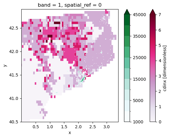
../../../_images/4fad1359b882ff48e007d35e041a2e61810a50498cad8bed437a0f76058bd6da.png

This plot doesn’t really help us doing climate risk assessemnt, so we can try to make a few changes to the map.

Custom plot#

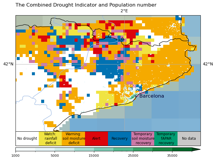
fig = plt.figure(figsize=(8, 6))
ax = fig.add_subplot(1, 1, 1, projection=ccrs.PlateCarree())

ax.set_extent([xmin, xmax, ymin, ymax], crs=ccrs.PlateCarree())

ax.stock_img()

# Plot CDI data
cmap = mpl.colors.ListedColormap(["#ffffff", "#f0e442", "#f5aa00", "#dc050c","#0072b2","#cc79a7","#009e73", "#c8c8c8"])
c = catalonia_cdi_latlon.cdinx.plot(ax=ax, cmap=cmap, vmin=-0.5, vmax=7.5, add_colorbar=False, add_labels=False)

#Plot the population
p_levels = [ 1000, 2500, 5000, 10000, 15000, 20000, 25000, 30000, 35000, 40000]
p = catalonia_population.plot(ax=ax, cmap=plt.cm.BuGn, levels=p_levels, extend='max', add_colorbar=False, add_labels=False)

# Customize gridlines
gridlines = p.axes.gridlines(draw_labels=True, dms=False, xlocs=[0, 2, 4], ylocs=[40, 42])
ax.add_feature(cfeature.BORDERS)
ax.add_feature(cfeature.COASTLINE)
ax.add_feature(cfeature.RIVERS)

plt.title('The Combined Drought Indicator and Population number', loc = "left")

#population colorbar
cax_p = fig.add_axes([ax.get_position().x0,
                    ax.get_position().y0-0.03,
                    ax.get_position().width,
                    0.02])
cbar_p = plt.colorbar(p, orientation="horizontal", cax=cax_p, ticks=[1000, 5000, 15000, 25000, 35000])
cbar_p.ax.tick_params(labelsize=8)

# CDI colorbar
cax_c = fig.add_axes([ax.get_position().x0,
                    ax.get_position().y0,
                    ax.get_position().width,
                    0.08])
cbar_c = plt.colorbar(c, orientation="horizontal", cax=cax_c)
cbar_c.ax.get_xaxis().set_ticks([])
for j, lab in enumerate(['No drought', 'Watch:\n rainfall\n deficit', 'Warning:\n soil moisture\n deficit', 'Alert','Recovery','Temporary\n soil moisture\n recovery','Temporary\n fAPAR\n recovery','No data']):
    cbar_c.ax.text(j, .5, lab, ha='center', va='center', size=8.5)

#text
barcelona_lon, barcelona_lat = 2.1686, 41.3874
text_kwargs = dict(fontsize=12, color='#000032', transform=ccrs.PlateCarree())
p.axes.text(barcelona_lon, barcelona_lat, '+ Barcelona', horizontalalignment='left', **text_kwargs)

Text(2.1686, 41.3874, '+ Barcelona')

../../../_images/5d534bcfcf906869fab6e9d97c6ab2301add9db0d263af43d391b98d16e728ce.png

Conclusions#

In this workflow, we have seen how to explore, process and visualise the data needed to analyse drought and population data.

Contributors#

Milana Vuckovic, ECMWF
Maurizio Mazzoleni, Vrije Universiteit Amsterdam

Appendix I - Customised plot explained step by step#

We will:

Add coastlines, rivers and country borders using cartopy
Set distinct colour levels for CDI
Remove the default colorbar and labels
Add custom colorbars and title
Add custom gridlines
And finally add a label for Barcelona

Background#

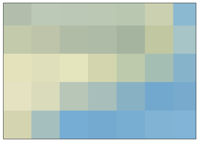
First we make a basic plot and set geographical extent to our domain. This way we can zoom in without having to manipulate the data.
We can also add some (low resolution) background.

fig = plt.figure(figsize=(8, 6))
ax = fig.add_subplot(1, 1, 1, projection=ccrs.PlateCarree())

ax.set_extent([xmin, xmax, ymin, ymax], crs=ccrs.PlateCarree())

# Add background image with orography
ax.stock_img()

<matplotlib.image.AxesImage at 0x19267ec50>

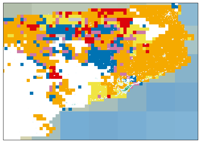
../../../_images/8a116cbb680ac7df949299c9d5aa6b64d722d9ead43e608d45aacb866aa7667c.png

Adding the data#

Next we add the data.
Here we customize the levels on both plots. We will also remove the default colorbar and labels, so in the next step we can add our own.

fig = plt.figure(figsize=(8, 6))
ax = fig.add_subplot(1, 1, 1, projection=ccrs.PlateCarree())

ax.set_extent([xmin, xmax, ymin, ymax], crs=ccrs.PlateCarree())

ax.stock_img()
#----------- New code to plot the data -----------#
# Plot CDI data
cmap = mpl.colors.ListedColormap(["#ffffff", "#f0e442", "#f5aa00", "#dc050c","#0072b2","#cc79a7","#009e73", "#c8c8c8"])
c = catalonia_cdi_latlon.cdinx.plot(ax=ax, cmap=cmap, vmin=-0.5, vmax=7.5, add_colorbar=False, add_labels=False)

#Plot the population
p_levels = [ 1000, 2500, 5000, 10000, 15000, 20000, 25000, 30000, 35000, 40000]
p = catalonia_population.plot(ax=ax, cmap=plt.cm.BuGn, levels=p_levels, extend='max', add_colorbar=False, add_labels=False)

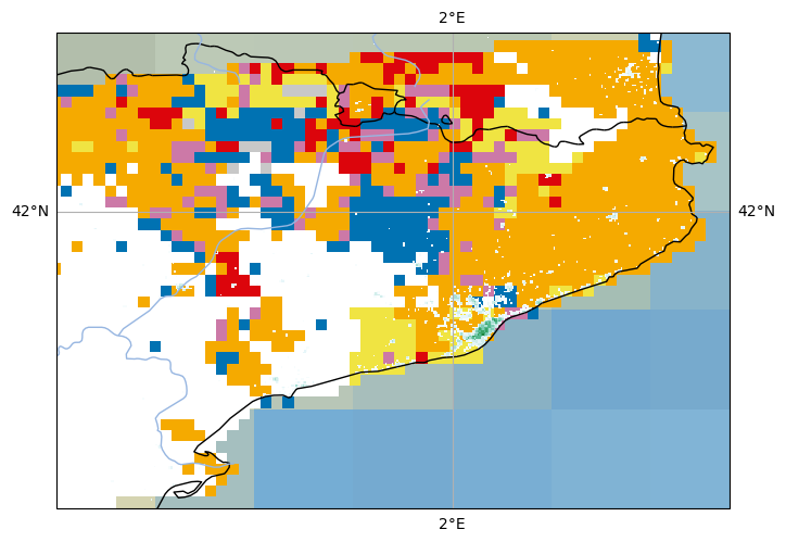
../../../_images/b0a7043be048710a44382052f3533b9e0198f92a2206b0288ea4a6aab3f51028.png

Adding the geographical features#

Next we add the gridlines, coastlines, rivers and country borders.

fig = plt.figure(figsize=(8, 6))
ax = fig.add_subplot(1, 1, 1, projection=ccrs.PlateCarree())

ax.set_extent([xmin, xmax, ymin, ymax], crs=ccrs.PlateCarree())

ax.stock_img()

# Plot CDI data
cmap = mpl.colors.ListedColormap(["#ffffff", "#f0e442", "#f5aa00", "#dc050c","#0072b2","#cc79a7","#009e73", "#c8c8c8"])
c = catalonia_cdi_latlon.cdinx.plot(ax=ax, cmap=cmap, vmin=-0.5, vmax=7.5, add_colorbar=False, add_labels=False)

#Plot the population
p_levels = [ 1000, 2500, 5000, 10000, 15000, 20000, 25000, 30000, 35000, 40000]
p = catalonia_population.plot(ax=ax, cmap=plt.cm.BuGn, levels=p_levels, extend='max', add_colorbar=False, add_labels=False)

#----------- New code to customize gridlines -----------#

gridlines = p.axes.gridlines(draw_labels=True, dms=False, xlocs=[0, 2, 4], ylocs=[40, 42])
ax.add_feature(cfeature.BORDERS)
ax.add_feature(cfeature.COASTLINE)
ax.add_feature(cfeature.RIVERS)

<cartopy.mpl.feature_artist.FeatureArtist at 0x19251c3d0>

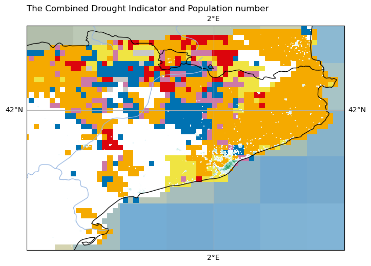
../../../_images/93bf08e0b9f9aa79023345d28ca021d4580385995548743a0d77399ce387bc78.png

Adding the title#

Then we add the title.

fig = plt.figure(figsize=(8, 6))
ax = fig.add_subplot(1, 1, 1, projection=ccrs.PlateCarree())

ax.set_extent([xmin, xmax, ymin, ymax], crs=ccrs.PlateCarree())

ax.stock_img()

# Plot CDI data
cmap = mpl.colors.ListedColormap(["#ffffff", "#f0e442", "#f5aa00", "#dc050c","#0072b2","#cc79a7","#009e73", "#c8c8c8"])
c = catalonia_cdi_latlon.cdinx.plot(ax=ax, cmap=cmap, vmin=-0.5, vmax=7.5, add_colorbar=False, add_labels=False)

#Plot the population
p_levels = [ 1000, 2500, 5000, 10000, 15000, 20000, 25000, 30000, 35000, 40000]
p = catalonia_population.plot(ax=ax, cmap=plt.cm.BuGn, levels=p_levels, extend='max', add_colorbar=False, add_labels=False)

# Customize gridlines
gridlines = p.axes.gridlines(draw_labels=True, dms=False, xlocs=[0, 2, 4], ylocs=[40, 42])
ax.add_feature(cfeature.BORDERS)
ax.add_feature(cfeature.COASTLINE)
ax.add_feature(cfeature.RIVERS)

#----------- New code to add the title -----------#

plt.title('The Combined Drought Indicator and Population number', loc = "left")

Text(0.0, 1.0, 'The Combined Drought Indicator and Population number')

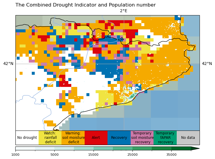
../../../_images/924030141f6345a5b6eddaa2867f76c46091c4e045f89b38299f905c6e58c5d9.png

Adding the colorbar#

It is a little bit tricky to add colorbars to where we want them.
cax_p and cax_c variable define the positions and size of the colorbars. They get the default position and size of the colorbars and make them half as long and next to each other.
In the end we also make the tick labels smaller.

fig = plt.figure(figsize=(8, 6))
ax = fig.add_subplot(1, 1, 1, projection=ccrs.PlateCarree())

ax.set_extent([xmin, xmax, ymin, ymax], crs=ccrs.PlateCarree())

ax.stock_img()

# Plot CDI data
cmap = mpl.colors.ListedColormap(["#ffffff", "#f0e442", "#f5aa00", "#dc050c","#0072b2","#cc79a7","#009e73", "#c8c8c8"])
c = catalonia_cdi_latlon.cdinx.plot(ax=ax, cmap=cmap, vmin=-0.5, vmax=7.5, add_colorbar=False, add_labels=False)

#Plot the population
p_levels = [ 1000, 2500, 5000, 10000, 15000, 20000, 25000, 30000, 35000, 40000]
p = catalonia_population.plot(ax=ax, cmap=plt.cm.BuGn, levels=p_levels, extend='max', add_colorbar=False, add_labels=False)



# Customize gridlines
gridlines = p.axes.gridlines(draw_labels=True, dms=False, xlocs=[0, 2, 4], ylocs=[40, 42])
ax.add_feature(cfeature.BORDERS)
ax.add_feature(cfeature.COASTLINE)
ax.add_feature(cfeature.RIVERS)

plt.title('The Combined Drought Indicator and Population number', loc = "left")

#----------- New code to add the horizontal colorbars -----------#

cax_p = fig.add_axes([ax.get_position().x0,
                    ax.get_position().y0-0.03,
                    ax.get_position().width,
                    0.02])
cbar_p = plt.colorbar(p, orientation="horizontal", cax=cax_p, ticks=[1000, 5000, 15000, 25000, 35000])
cbar_p.ax.tick_params(labelsize=8)

# CDI colorbar
cax_c = fig.add_axes([ax.get_position().x0,
                    ax.get_position().y0,
                    ax.get_position().width,
                    0.08])
cbar_c = plt.colorbar(c, orientation="horizontal", cax=cax_c)
cbar_c.ax.get_xaxis().set_ticks([])
for j, lab in enumerate(['No drought', 'Watch:\n rainfall\n deficit', 'Warning:\n soil moisture\n deficit', 'Alert','Recovery','Temporary\n soil moisture\n recovery','Temporary\n fAPAR\n recovery','No data']):
    cbar_c.ax.text(j, .5, lab, ha='center', va='center', size=8.5)

../../../_images/17176b55165be8bfd120ca51be4c420e7f6e56015ca79c8f91705c6410021dc6.png

Adding the custom text label#

Finally we can add the label for Barcelona.

fig = plt.figure(figsize=(8, 6))
ax = fig.add_subplot(1, 1, 1, projection=ccrs.PlateCarree())

ax.set_extent([xmin, xmax, ymin, ymax], crs=ccrs.PlateCarree())

ax.stock_img()

# Plot CDI data
cmap = mpl.colors.ListedColormap(["#ffffff", "#f0e442", "#f5aa00", "#dc050c","#0072b2","#cc79a7","#009e73", "#c8c8c8"])
c = catalonia_cdi_latlon.cdinx.plot(ax=ax, cmap=cmap, vmin=-0.5, vmax=7.5, add_colorbar=False, add_labels=False)

#Plot the population
p_levels = [ 1000, 2500, 5000, 10000, 15000, 20000, 25000, 30000, 35000, 40000]
p = catalonia_population.plot(ax=ax, cmap=plt.cm.BuGn, levels=p_levels, extend='max', add_colorbar=False, add_labels=False)



# Customize gridlines
gridlines = p.axes.gridlines(draw_labels=True, dms=False, xlocs=[0, 2, 4], ylocs=[40, 42])
ax.add_feature(cfeature.BORDERS)
ax.add_feature(cfeature.COASTLINE)
ax.add_feature(cfeature.RIVERS)

plt.title('The Combined Drought Indicator and Population number', loc = "left")

cax_p = fig.add_axes([ax.get_position().x0,
                    ax.get_position().y0-0.03,
                    ax.get_position().width,
                    0.02])
cbar_p = plt.colorbar(p, orientation="horizontal", cax=cax_p, ticks=[1000, 5000, 15000, 25000, 35000])
cbar_p.ax.tick_params(labelsize=8)

# CDI colorbar
cax_c = fig.add_axes([ax.get_position().x0,
                    ax.get_position().y0,
                    ax.get_position().width,
                    0.08])
cbar_c = plt.colorbar(c, orientation="horizontal", cax=cax_c)
cbar_c.ax.get_xaxis().set_ticks([])
for j, lab in enumerate(['No drought', 'Watch:\n rainfall\n deficit', 'Warning:\n soil moisture\n deficit', 'Alert','Recovery','Temporary\n soil moisture\n recovery','Temporary\n fAPAR\n recovery','No data']):
    cbar_c.ax.text(j, .5, lab, ha='center', va='center', size=8.5)

#----------- New code to add the text annotation -----------#

barcelona_lon, barcelona_lat = 2.1686, 41.3874
text_kwargs = dict(fontsize=12, color='#000032', transform=ccrs.PlateCarree())
p.axes.text(barcelona_lon, barcelona_lat, '+ Barcelona', horizontalalignment='left', **text_kwargs)

Text(2.1686, 41.3874, '+ Barcelona')

Simple droughts workflow

Contents

Simple droughts workflow#

Risk assessment methodology#

Two additional classes - namely

Preparation work#

Load libraries#

Create the directory structure#

Download data#

Population data#

The Combined Drought Indicator (CDI)#

Explore the data#

Population data#

The Combined Drought Indicator (CDI)#

Process the data#

Select the area of interest#

Plot it together#

Basic plot#

Custom plot#

Conclusions#

Contributors#

Appendix I - Customised plot explained step by step#

Background#

Adding the data#

Adding the geographical features#

Adding the title#

Adding the colorbar#

Adding the custom text label#