Potential coastal flood impacts#
Risk assessment methodology#
In this workflow we will consider the potential impacts of coastal flooding caused by extreme sea water levels. The methodology of calculating the flood risk is similar to that of the river flooding workflow (link). The flood risk is calculated based on flood maps and economic damage functions. The flood maps are considered for two climates: present day climate (ca. 2018) and 2050 (under RCP8.5 climate scenario). For each climate, different return periods of the extreme conditions are considered.
The following datasets are used as input for the calculations:
Flood maps: the maps of flood depth (coastal inundation depth) are based on the Global Flood Maps dataset openly available via the Microsoft Planetary Computer (link to dataset).
Land-use information: The land cover map is available from the Copernicus Land Monitoring Service.
Damage curves expressed as relative damage percentage (available here
The output of this calculation is the flood damage maps per scenario. Flood damage is calculated by applying damage curves to the flood inundation depth maps, taking into account the local situation. For each grid point, the damage is calculated based on the flood depth, land use type, damage curves, and country-specific parameters (can be defined by the user) that approximate the economic value of different land use types.
Description of the coastal flood map dataset and its limitations#
The Global Flood Maps dataset was developed by Deltares based on global modelling of water levels that are affected by tides, storm surges and sea level rise. In this dataset, maps for present climate (ca. 2018) and future climate (ca. 2050) are available, with extreme water levels corresponding to return periods of 2, 5, 10, 25, 50, 100 and 250 years. The 2050 scenario assumes sea level rise as estimated under RCP8.5 (high-emission scenario). The flood maps have a resolution of 3 arcseconds (30-75 m in European geographical area, depending on latitude).
The methodology behind this dataset is documented and can be accessed on the (main page). The dataset is based on the GTSMv3.0 (Global Tide and Surge model), forced with ERA5 atmospheric dataset. Statistical analysis of modelled data is used to arrive at extreme water level values for different return periods. These values are used to calculate flood depths by applying static inundation modelling routine (“bathtub” method, with a simplified correction for friction over land) over a high-resolution Digital Elevation Model (MERIT-DEM or NASADEM).
Several things to take into account when interpreting the flood maps:
This dataset helps to understand the coastal flood potential at a given location. The flood modelling in this dataset does not account for man-made coastal protections that may already be in place in populated regions (e.g. dams, storm barriers). Therefore, it is always important to survey the local circumstances when interpreting the flood maps.
The resolution of this global dataset is very high, when considered on a global scale. However, for local areas with complex bathymetries the performance of the models is likely reduced (e.g. in estuaries or semi-enclosed bays) and the results should be treated with caution.
For a more accurate estimate of coastal flood risks, it is recommended to perform local flood modelling, taking the results of the global model as boundary conditions. Local models can take better account of complex bathymetry and topography, and incorporate local data and knowledge about e.g. flood protection measures.
Preparation work#
Load libraries#
In this notebook we will use the following Python libraries:
os - Provides a way to interact with the operating system, allowing the creation of directories and file manipulation.
pooch - A data retrieval and storage utility that simplifies downloading and managing datasets.
numpy - A powerful library for numerical computations in Python, widely used for array operations and mathematical functions.
pandas - A data manipulation and analysis library, essential for working with structured data in tabular form.
rasterio - A library for reading and writing geospatial raster data, providing functionalities to explore and manipulate raster datasets.
rioxarray - An extension of the xarray library that simplifies working with geospatial raster data in GeoTIFF format.
damagescanner - A library designed for calculating flood damages based on geospatial data, particularly suited for analyzing flood impact.
matplotlib - A versatile plotting library in Python, commonly used for creating static, animated, and interactive visualizations.
contextily A library for adding basemaps to plots, enhancing geospatial visualizations.
cartopy A library for geospatial data processing.
planetary-computer A library for interacting with the Microsoft Planetary Computer.
dask A library for parallel computing and task scheduling.
pystac-client A library for for working with STAC Catalogs and APIs.
shapely A library for manipulation and analysis of geometric objects.
These libraries collectively enable the download, processing, analysis, and visualization of geospatial and numerical data.
# Package for downloading data and managing files
import os
import pooch
import dask.distributed
import pystac_client
import planetary_computer

# Packages for working with numerical data and tables
import numpy as np
import pandas as pd

# Packages for handling geospatial maps and data
import rioxarray as rxr
from rioxarray.merge import merge_datasets
import xarray as xr
import rasterio
from rasterio.enums import Resampling

# Package for calculating flood damages
from damagescanner.core import RasterScanner

# Ppackages used for plotting maps
import matplotlib.pyplot as plt
import contextily as ctx
import shapely.geometry
import cartopy.feature as cfeature
import cartopy.crs as ccrs
Select area of interest#
Before downloading the data, we will define the coordinates of the area of interest. Based on these coordinates we will be able to clip the datasets for further processing, and eventually display hazard and damage maps for the selected area.
To easily define an area in terms of geographical coordinates, you can go to the Bounding Box Tool to select a region and get the coordinates. Make sure to select ‘CSV’ in the lower left corner and copy the values in the brackets below. Next to coordinates, please specify a name for the area which will be used in plots and saved results.
bbox = [-2.94,51.4,-2.5,51.7]; areaname = 'Bristol'

#bbox = [1.983871,41.252461,2.270614,41.449569]; areaname = 'Barcelona'
#bbox = [-1.6,46,-1.05,46.4]; areaname = 'La_Rochelle'
#bbox = [12.1,45.1,12.6,45.7]; areaname = 'Venice'
Create the directory structure#
# Define the folder for the flood workflow
workflow_folder = 'coastal_flood_workflow'

# Check if the workflow folder exists, if not, create it along with subfolders for data and results
if not os.path.exists(workflow_folder):
    os.makedirs(workflow_folder)
    os.makedirs(os.path.join(workflow_folder, 'data'))
    os.makedirs(os.path.join(workflow_folder, f'results_{areaname}'))
# Define directories for data and results within the previously defined workflow folder
data_dir = os.path.join(workflow_folder, 'data')
results_dir = os.path.join(workflow_folder, f'results_{areaname}')
Download data#
Flood map data#
We will use the potential coastal flood depth maps from the Global Flood Maps dataset, which is accessible remotely via API. Below we will first explore an example of a flood map from the dataset, and then load a subset of this dataset for our area of interest.
# prepare to connect to server
client = dask.distributed.Client(processes=False)
print(client.dashboard_link)
http://192.168.178.80:8787/status
# establish connection and search for floodmaps
catalog = pystac_client.Client.open(
    "https://planetarycomputer.microsoft.com/api/stac/v1",
    modifier=planetary_computer.sign_inplace,
)
search = catalog.search(
    collections=["deltares-floods"],
    query={
        "deltares:dem_name": {"eq": "MERITDEM"},         # option to select the underlying DEM (MERITDEM or NASADEM)
        "deltares:resolution": {"eq": '90m'}})           # option to select resolution (recommended: 90m)

# Print the all found items:
#for item in search.items():
#    print(item.id)

# Print the first item
print(next(search.items()))

# count the number of items
items = list(search.items())
print("Number of items found: ",len(items))
<Item id=MERITDEM-90m-2050-0250>
Number of items found:  16
In the cell above, connection to the server was made and a list of all items that match our search was retrieved. Here the search was restricted to one Digital Elevation Model (MERIT-DEM) with high-resolution maps (90 m at equator). The first item of the list was printed to check correctness of the search, displaying the “item ID” in the format of {DEM name}-{resolution}-{year}-{return period}. The total number of records is also printed, which includes all available combinations of scenario years (2018 or 2050) and extreme water level return periods.
Now we will select the first item as an example and process it to view the flood map.
# select first item from the search and open the dataset
item = next(search.items())
url = item.assets["index"].href
ds = xr.open_dataset(f"reference::{url}", engine="zarr", consolidated=False, chunks={})
We have opened the first dataset. The extent of the dataset is global, therefore the number of points along latitude and longitude axes is very large. This dataset needs to be clipped to our area of interest, reprojected to local coordinates.
We can view the contents of the raw dataset:
print(ds)
<xarray.Dataset>
Dimensions:     (time: 1, lat: 216000, lon: 432000)
Coordinates:
  * lat         (lat) float64 -90.0 -90.0 -90.0 -90.0 ... 90.0 90.0 90.0 90.0
  * lon         (lon) float64 -180.0 -180.0 -180.0 -180.0 ... 180.0 180.0 180.0
  * time        (time) datetime64[ns] 2010-01-01
Data variables:
    inun        (time, lat, lon) float32 dask.array<chunksize=(1, 4000, 4000), meta=np.ndarray>
    projection  object ...
Attributes:
    Conventions:  CF-1.6
    config_file:  /mnt/globalRuns/watermask_post_MERIT/run_rp0250_slr2050/coa...
    institution:  Deltares
    project:      Microsoft Planetary Computer - Global Flood Maps
    references:   https://www.deltares.nl/en/
    source:       Global Tide and Surge Model v3.0 - ERA5
    title:        GFM - MERIT DEM 90m - 2050 slr - 0250-year return level
Now we will clip the dataset to a wider area around the region of interest, and call it ds_local. The extra margin is added to account for reprojection at a later stage. The clipping of the dataset allows to reduce the total size of the dataset so that it can be loaded into memory for faster processing and plotting.
ds_local = ds.sel(lat=slice(bbox[1]-0.5,bbox[3]+0.5), lon=slice(bbox[0]-0.5,bbox[2]+0.5),drop=True).squeeze(); del ds
ds_local.load()
<xarray.Dataset>
Dimensions:     (lat: 1561, lon: 1728)
Coordinates:
  * lat         (lat) float64 50.9 50.9 50.9 50.9 50.9 ... 52.2 52.2 52.2 52.2
  * lon         (lon) float64 -3.439 -3.438 -3.438 -3.437 ... -2.002 -2.001 -2.0
    time        datetime64[ns] 2010-01-01
Data variables:
    inun        (lat, lon) float32 0.0 0.0 0.0 0.0 0.0 ... 0.0 0.0 0.0 0.0 0.0
    projection  object nan
Attributes:
    Conventions:  CF-1.6
    config_file:  /mnt/globalRuns/watermask_post_MERIT/run_rp0250_slr2050/coa...
    institution:  Deltares
    project:      Microsoft Planetary Computer - Global Flood Maps
    references:   https://www.deltares.nl/en/
    source:       Global Tide and Surge Model v3.0 - ERA5
title: GFM - MERIT DEM 90m - 2050 slr - 0250-year return levelWe will convert the dataset to a geospatial array, drop the unnecessary coordinates, reproject the array to the projected coordinate system for Europe, and, finally, clip it to the region of interest using our bounding box.
ds_local.rio.write_crs(ds_local.projection.EPSG_code, inplace=True)
ds_local = ds_local.drop_vars({"projection","time"})
ds_local = ds_local.rio.reproject("epsg:3035")
ds_local = ds_local.rio.clip_box(*bbox, crs="EPSG:4326")
We can now plot the dataset to see the flood map for one scenario and return period:
fig, ax = plt.subplots(figsize=(7, 7))
bs=ds_local.where(ds_local.inun>0)['inun'].plot(ax=ax,cmap='Blues',alpha=1)
ctx.add_basemap(ax=ax,crs='EPSG:3035',source=ctx.providers.CartoDB.Positron, attribution_size=6)
plt.title(f'Example of a floodmap retrieved for the area of {areaname} \n {ds_local.attrs["title"]}',fontsize=12);

We would like to be able to compare the flood maps for different scenarios and return periods. For this, we will load and merge the datasets for different scenarios and return periods in one dataset, where the flood maps can be easily accessed. Below a function is defined which contains the steps described above for an individual dataset.
# combine the above steps into a function to load flood maps per year and return period
def load_floodmaps(catalog,year,rp):
    search = catalog.search(
    collections=["deltares-floods"],
    query={
        "deltares:dem_name": {"eq": "MERITDEM"},
        "deltares:resolution": {"eq": '90m'},
        "deltares:sea_level_year": {"eq": year},
        "deltares:return_period": {"eq": rp}})
    item=next(search.items())
    url = item.assets["index"].href
    ds = xr.open_dataset(f"reference::{url}", engine="zarr", consolidated=False, chunks={})
    ds_local = ds.sel(lat=slice(bbox[1]-0.5,bbox[3]+0.5), lon=slice(bbox[0]-0.5,bbox[2]+0.5),drop=True).squeeze(); del ds
    ds_local.load()
    ds_local.rio.write_crs(ds_local.projection.EPSG_code, inplace=True)
    ds_local = ds_local.drop_vars({"projection","time"})
    ds_local = ds_local.rio.reproject("epsg:3035")
    ds_local = ds_local.rio.clip_box(*bbox, crs="EPSG:4326")
    ds_local = ds_local.assign_coords(year=year); ds_local = ds_local.expand_dims('year') # write corresponding scenario year in the dataset coordinates
    ds_local = ds_local.assign_coords(return_period=rp); ds_local = ds_local.expand_dims('return_period') # write corresponding return period in the dataset coordinates
    ds_floodmap = ds_local.where(ds_local.inun > 0); del ds_local
    return ds_floodmap
We can now apply this function, looping over the two scenarios and a selection of return periods.
In the Global Flood Maps dataset there are two climate scenarios: present day (represented by the year 2018) and future (year 2050, with sea level rise corresponding to the high-emission scenario, RCP8.5). The available return periods range between 2 years and 250 years. Below we make a selection that includes 5, 10, 50, 100-year return periods).
# load all floodmaps in one dataset
years = [2018,2050] # list of scenario years (2018 and 2050)
rps = [2,5,10,50,100,250] # list of return periods (all: 2,5,10,25,50,100,250 yrs)
for year in years:
    for rp in rps:
        ds = load_floodmaps(catalog,year,rp)
        if (year==years[0]) & (rp==rps[0]):
            floodmaps = ds
        else:
            floodmaps = xr.merge([floodmaps,ds],combine_attrs="drop_conflicts")
        del ds
The floodmaps variable now contains the flood maps for different years and scenarios. We can view the contents of the variable:
print(floodmaps)
<xarray.Dataset>
Dimensions:        (x: 474, y: 506, year: 2, return_period: 6)
Coordinates:
  * x              (x) float64 3.426e+06 3.426e+06 ... 3.462e+06 3.462e+06
  * y              (y) float64 3.256e+06 3.256e+06 ... 3.218e+06 3.218e+06
  * year           (year) int32 2018 2050
  * return_period  (return_period) int32 2 5 10 50 100 250
    spatial_ref    int32 0
Data variables:
    inun           (return_period, year, y, x) float32 nan nan nan ... nan nan
Attributes:
    Conventions:  CF-1.6
    institution:  Deltares
    project:      Microsoft Planetary Computer - Global Flood Maps
    references:   https://www.deltares.nl/en/
    source:       Global Tide and Surge Model v3.0 - ERA5
We will use the dataset in the floodmaps variable later on in this workflow to calculate flood risk.
Land-use information#
Next we need the information on land use. We will download the land use dataset from the JRC data portal, a copy of the dataset will be saved locally for ease of access.
landuse_res = 50 # choose resolution (options: 50 or 100 m)
luisa_filename = f'LUISA_basemap_020321_{landuse_res}m.tif'

# Check if land use dataset has not yet been downloaded
if  not os.path.isfile(os.path.join(data_dir,luisa_filename)):
    # , define the URL for the LUISA basemap and download it
    url = f'http://jeodpp.jrc.ec.europa.eu/ftp/jrc-opendata/LUISA/EUROPE/Basemaps/2018/VER2021-03-24/{luisa_filename}'
    pooch.retrieve(
        url=url,
        known_hash=None,  # Hash value is not provided
        path=data_dir,    # Save the file to the specified data directory
        fname=luisa_filename  # Save the file with a specific name
    )
else:
    print(f'Land use dataset already downloaded at {data_dir}/{luisa_filename}')
Land use dataset already downloaded at coastal_flood_workflow\data/LUISA_basemap_020321_100m.tif
The Land use data is extracted into the local data directory. The data shows on a 100 by 100 meter resolution what the land use is for Europe in 2018. The land use encompasses various types of urban areas, natural land, agricultural fields, infrastructure and waterbodies. This will be used as the exposure layer in the risk assessment.
# Define the filename for the land use map based on the specified data directory
filename_land_use = f'{data_dir}/{luisa_filename}'

# Open the land use map raster using rioxarray
land_use = rxr.open_rasterio(filename_land_use)

# Display the opened land use map
print(land_use)
<xarray.DataArray (band: 1, y: 46000, x: 65000)>
[2990000000 values with dtype=int32]
Coordinates:
  * band         (band) int32 1
  * x            (x) float64 9e+05 9.002e+05 9.002e+05 ... 7.4e+06 7.4e+06
  * y            (y) float64 5.5e+06 5.5e+06 5.5e+06 ... 9.002e+05 9e+05
    spatial_ref  int32 0
Attributes:
    AREA_OR_POINT:  Area
    _FillValue:     0
    scale_factor:   1.0
    add_offset:     0.0
The land use dataset needs to be clipped to the area of interest. For visualization purposes, each land use type is then assigned a color. Land use plot shows us the variation in land use over the area of interest.
# Set the coordinate reference system (CRS) for the land use map to EPSG:3035
land_use.rio.write_crs(3035, inplace=True)

# Clip the land use map to the specified bounding box and CRS
land_use_local = land_use.rio.clip_box(*bbox, crs="EPSG:4326")

# File to store the local land use map
landuse_map = os.path.join(data_dir, f'land_use_{areaname}.tif')

# Save the clipped land use map
with rasterio.open(
    landuse_map,
    'w',
    driver='GTiff',
    height=land_use_.shape[1],
    width=land_use_.shape[2],
    count=1,
    dtype=str(land_use_local.dtype),
    crs=land_use_local.rio.crs,
    transform=land_use_local.rio.transform()
) as dst:
    # Write the data array values to the rasterio dataset
    dst.write(land_use_local.values)
# Plotting

# Define values and colors for different land use classes
LUISA_values = [1111, 1121, 1122, 1123, 1130,
                1210, 1221, 1222, 1230, 1241,
                1242, 1310, 1320, 1330, 1410,
                1421, 1422, 2110, 2120, 2130,
                2210, 2220, 2230, 2310, 2410,
                2420, 2430, 2440, 3110, 3120,
                3130, 3210, 3220, 3230, 3240,
                3310, 3320, 3330, 3340, 3350,
                4000, 5110, 5120, 5210, 5220,
                5230]

LUISA_colors = ["#8c0000", "#dc0000", "#ff6969", "#ffa0a0", "#14451a",
                "#cc10dc", "#646464", "#464646", "#9c9c9c", "#828282",
                "#4e4e4e", "#895a44", "#a64d00", "#cd8966", "#55ff00",
                "#aaff00", "#ccb4b4", "#ffffa8", "#ffff00", "#e6e600",
                "#e68000", "#f2a64d", "#e6a600", "#e6e64d", "#c3cd73",
                "#ffe64d", "#e6cc4d", "#f2cca6", "#38a800", "#267300",
                "#388a00", "#d3ffbe", "#cdf57a", "#a5f57a", "#89cd66",
                "#e6e6e6", "#cccccc", "#ccffcc", "#000000", "#ffffff",
                "#7a7aff", "#00b4f0", "#50dcf0", "#00ffa6", "#a6ffe6",
                "#e6f2ff"]

# Plot the land use map using custom levels and colors
land_use_local.plot(levels=LUISA_values, colors=LUISA_colors, figsize=(10, 10))

# Set the title for the plot
plt.title('LUISA Land Cover for the defined area')
Text(0.5, 1.0, 'LUISA Land Cover for the defined area')

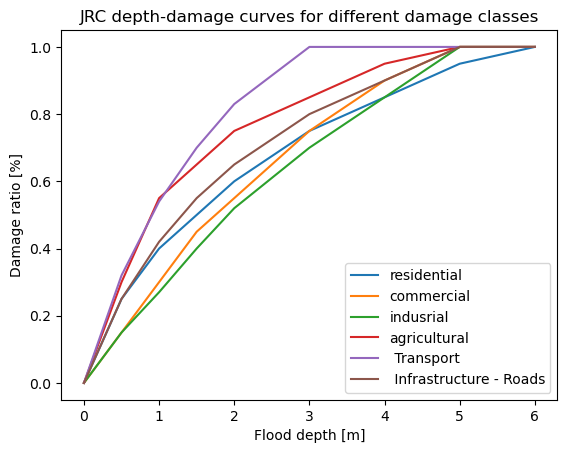
Damage curves#
We will use damage curve files from the JRC.
# Import damage curves of the JRC from a CSV file into a pandas DataFrame
JRC_curves = pd.read_csv('JRC_damage_curves.csv', index_col=0)

# Plot the JRC depth-damage curves
JRC_curves.plot()

# Set the title and labels for the plot
plt.title('JRC depth-damage curves for different damage classes')
plt.xlabel('Flood depth [m]')
plt.ylabel('Damage ratio [%]')
Text(0, 0.5, 'Damage ratio [%]')
Processing data: from hazard to risk#
The maps of flooding and land use can be combined to assess multipe types of risk from coastal flooding in a region. This way we can estimate the exposure of population, infrastructure and economic assets to coastal floods. Different methods exist for translating hazard maps to risk estimations. In this workflow we will look into estimating the potential economic damages.
Combining datasets with different resolution#
The flood and land use datasets have different spatial resolutions. Flood extent maps are at a resolution of 30-75 m (resolution varies with latitude), while land use data is at a constant 100 m resolution. We can bring them to the same resolution.
Both grids have a similar resolution, but it is preferable to interpolate the flood map onto the land use grid, because land use is defined in terms of discrete values and on a more convenient regularly spaced grid. We will interpolate the flood data onto the land use map grid in order to be able to calculate the damages.
# Reproject the flood map to match the resolution and extent of the land use map
for year in years:
    for rp in rps:
        ori_map = floodmaps['inun'].sel(year=year,return_period=rp)
        new_map = ori_map.rio.reproject_match(land_use_local, resampling=Resampling.bilinear); del ori_map
        ds = new_map.to_dataset(); del new_map
        ds = ds.expand_dims(dim={'year':1,'return_period':1})

        if (year==years[0]) & (rp==rps[0]):
            floodmaps_resampled = ds
        else:
            floodmaps_resampled = floodmaps_resampled.merge(ds)
# check the new resolution of the floodmap (should be equivalent to the land use map resolution)
floodmaps_resampled.rio.resolution()
(100.0, -100.0)
We will save the resampled flood maps in raster format locally, so that DamageScanner package can use them as input to calculate economic damages.
# Create GeoTIFF files for the resampled flood maps
tif_dir = os.path.join(data_dir,f'floodmap_plots_resampled_{areaname}')
if not os.path.isdir(tif_dir): os.makedirs(tif_dir)
for year in years:
    for rp in rps:
        data_tif = floodmaps_resampled['inun'].sel(year=year,return_period=rp,drop=True)
        with rasterio.open(
            f'{tif_dir}/floodmap_resampled_{areaname}_{year}_rp{rp:04d}.tif',
            'w',
            driver='GTiff',
            height=data_tif.shape[0],
            width=data_tif.shape[1],
            count=1,
            dtype=str(data_tif.dtype),
            crs=data_tif.rio.crs,
            transform=data_tif.rio.transform(),
        ) as dst:
            # Write the data array values to the rasterio dataset
            dst.write(data_tif.values,indexes=1)
Linking land use types to economic damages#
In order to assess the potential damage done by the flooding in a given scenario, we also need to assign a monetary value to the land use categories. We define this as the potential loss in €/m². Go into the provided LUISA_damage_info_curves.xlsx and tweak the information to your own region.
# Read damage curve information from an Excel file into a pandas DataFrame
LUISA_info_damage_curve = pd.read_excel('LUISA_damage_info_curves.xlsx', index_col=0)

# Extract the 'total €/m²' column to get the maximum damage for reconstruction
maxdam = pd.DataFrame(LUISA_info_damage_curve['total €/m²'])

# Save the maximum damage values to a CSV file
maxdam_path = os.path.join(data_dir, f'maxdam_luisa.csv')
maxdam.to_csv(maxdam_path)

# Display the first 10 rows of the resulting DataFrame to view the result
maxdam.head(10)
| total €/m² | |
|---|---|
| Land use code | |
| 1111 | 600.269784 |
| 1121 | 414.499401 |
| 1122 | 245.022999 |
| 1123 | 69.919184 |
| 1130 | 0.000000 |
| 1210 | 405.238393 |
| 1221 | 40.417363 |
| 1222 | 565.843080 |
| 1230 | 242.504177 |
| 1241 | 565.843080 |
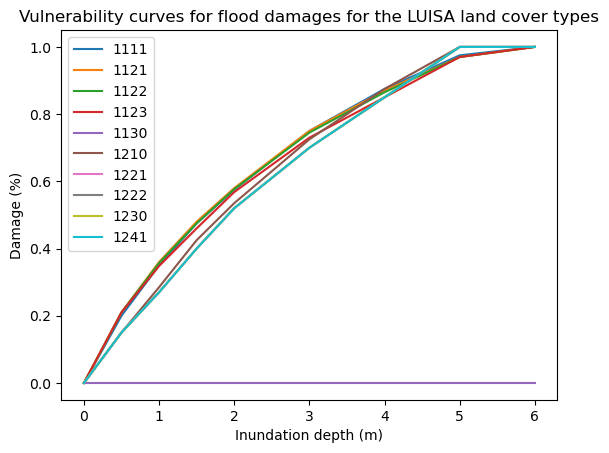
# Create a new DataFrame for damage_curves_luisa by copying JRC_curves
damage_curves_luisa = JRC_curves.copy()

# Drop all columns in the new DataFrame
damage_curves_luisa.drop(damage_curves_luisa.columns, axis=1, inplace=True)

# Define building types for consideration
building_types = ['residential', 'commercial', 'industrial']

# For each land use class in maxdamage, create a new damage curve
for landuse in maxdam.index:
    # Find the ratio of building types in the class
    ratio = LUISA_info_damage_curve.loc[landuse, building_types].values

    # Create a new curve based on the ratios and JRC_curves
    damage_curves_luisa[landuse] = ratio[0] * JRC_curves.iloc[:, 0] + \
                                   ratio[1] * JRC_curves.iloc[:, 1] + \
                                   ratio[2] * JRC_curves.iloc[:, 2]

# Save the resulting damage curves to a CSV file
curve_path = os.path.join(data_dir, 'curves.csv')
damage_curves_luisa.to_csv(curve_path)

# Plot the vulnerability curves for the first 10 land cover types
damage_curves_luisa.iloc[:, 0:10].plot()
plt.title('Vulnerability curves for flood damages for the LUISA land cover types')
plt.ylabel('Damage (%)')
plt.xlabel('Inundation depth (m)')
Text(0.5, 0, 'Inundation depth (m)')
Calculate potential damage using DamageScanner#
Now that we have all pieces of the puzzle in place, we can perform the risk calculation. For this we are using the DamageScanner python library which allows for an easy damage calculation.
The DamageScanner takes the following data:
The clipped and resampled flood map
The clipped landuse map
The vulnerability curves per land use category
A table of maximum damages per land use category
We can perform the damage calculations for all scenarios and return periods now:
for year in years:
    for rp in rps:
        inun_map = os.path.join(tif_dir, f'floodmap_resampled_{areaname}_{year}_rp{rp:04}.tif') # Define file path for the flood map input

        # Do the damage calculation and save the results
        loss_df = RasterScanner(landuse_map,
                                inun_map,
                                curve_path,
                                maxdam_path,
                                save = True,
                                nan_value = None,
                                scenario_name= '{}/flood_scenario_{}_{}_rp{:04}'.format(results_dir,areaname,year,rp),
                                dtype = np.int64)
        loss_df_renamed = loss_df[0].rename(columns={"damages": "{}_rp{:04}".format(year,rp)})

        if (year==years[0]) & (rp==rps[0]):
            loss_df_all = loss_df_renamed
        else:
            loss_df_all = pd.concat([loss_df_all, loss_df_renamed], axis=1)
Now the dataframe loss_df_all contains the results of damage calculations for all scenarios and return periods. We will format this dataframe for easier interpretation:
# Obtain the LUISA legend and add it to the table of damages
LUISA_legend = LUISA_info_damage_curve['Description']

# Convert the damages to million euros
loss_df_all_mln = loss_df_all / 10**6

# Combine loss_df with LUISA_legend
category_damage = pd.concat([LUISA_legend, (loss_df_all_mln)], axis=1)

# Sort the values by damage in descending order (based on the column with the highest damages)
category_damage.sort_values(by='2050_rp0250', ascending=False, inplace=True)

# Display the resulting DataFrame (top 10 rows)
category_damage.head(10)
| Description | 2018_rp0002 | 2018_rp0005 | 2018_rp0010 | 2018_rp0050 | 2018_rp0100 | 2018_rp0250 | 2050_rp0002 | 2050_rp0005 | 2050_rp0010 | 2050_rp0050 | 2050_rp0100 | 2050_rp0250 | |
|---|---|---|---|---|---|---|---|---|---|---|---|---|---|
| 1210 | Industrial or commercial units | 1000.517647 | 1529.168675 | 2073.110967 | 3516.429868 | 4118.944877 | 4930.327871 | 1231.567959 | 1823.617944 | 2401.923540 | 3831.457751 | 4478.271172 | 5233.549132 |
| 2310 | Pastures | 1829.850119 | 2229.676585 | 2500.199547 | 3048.992169 | 3257.661892 | 3523.235250 | 2008.426032 | 2385.241506 | 2637.764313 | 3169.420519 | 3376.428448 | 3630.917261 |
| 2110 | Non irrigated arable land | 792.849411 | 1027.744061 | 1179.846847 | 1497.963143 | 1611.379646 | 1756.081620 | 902.812690 | 1114.464226 | 1261.257438 | 1562.652179 | 1673.913869 | 1820.228496 |
| 1121 | Medium density urban fabric | 251.266262 | 490.326773 | 701.191945 | 1067.704658 | 1191.197005 | 1378.829691 | 342.664542 | 593.331993 | 774.817075 | 1129.077454 | 1273.477108 | 1470.541448 |
| 1123 | Isolated or very low density urban fabric | 108.070598 | 144.510086 | 168.141687 | 235.083132 | 258.596272 | 289.547197 | 121.827843 | 158.512160 | 187.133728 | 248.857176 | 270.765426 | 301.775546 |
| 1111 | High density urban fabric | 1.019247 | 10.885994 | 45.226896 | 155.902570 | 191.716769 | 228.450762 | 8.919931 | 21.982771 | 63.363088 | 178.980802 | 203.395169 | 247.141392 |
| 1230 | Port areas | 15.244354 | 23.607465 | 34.840021 | 83.281079 | 112.992847 | 185.733999 | 18.096094 | 30.369824 | 48.127132 | 98.404765 | 154.675885 | 228.031683 |
| 1122 | Low density urban fabric | 80.830840 | 120.529666 | 135.502403 | 176.181251 | 188.198476 | 211.019285 | 98.582201 | 128.912025 | 144.411329 | 183.169715 | 196.083244 | 217.234946 |
| 1330 | Construction sites | 70.281220 | 95.036155 | 114.606479 | 157.105919 | 174.627202 | 193.914805 | 81.291668 | 107.503344 | 131.266075 | 168.928411 | 181.924748 | 206.668312 |
| 1221 | Road and rail networks and associated land | 40.014690 | 54.790595 | 67.312664 | 95.938364 | 108.128946 | 125.184446 | 46.429911 | 62.355269 | 74.171976 | 103.313669 | 116.685205 | 133.884823 |
Plot the results#
Now we can plot the damages to get a spatial view of what places can potentially be most affected economically. To do this, first the damage maps for all scenarios will be loaded into memory and formatted:
# load all damage maps and merge into one dataset
for year in years:
    for rp in rps:
        damagemap = rxr.open_rasterio('{}/flood_scenario_{}_{}_rp{:04}_damagemap.tif'.format(results_dir,areaname,year,rp)).squeeze()
        damagemap = damagemap.where(damagemap > 0)/10**6
        damagemap.load()

        # prepare for merging
        damagemap.name = 'damages'
        damagemap = damagemap.assign_coords(year=year);
        damagemap = damagemap.assign_coords(return_period=rp);
        ds = damagemap.to_dataset(); del damagemap
        ds = ds.expand_dims(dim={'year':1,'return_period':1})

        # merge
        if (year==years[0]) & (rp==rps[0]):
            damagemap_all = ds
        else:
            damagemap_all = damagemap_all.merge(ds)
damagemap_all.x.attrs['long_name'] = 'X coordinate'; damagemap_all.x.attrs['units'] = 'm'
damagemap_all.y.attrs['long_name'] = 'Y coordinate'; damagemap_all.y.attrs['units'] = 'm'
damagemap_all.load()
Now we can plot the damage maps to compare:
# Plot damage maps for different scenarios and return periods
fig,axs = plt.subplots(figsize=(20, 8),nrows=len(years),ncols=len(rps),constrained_layout=True,sharex=True,sharey=True)

# define limits for the damage axis based on the map with highest damages
vrange = [0,np.nanmax(damagemap_all.sel(year=2050,return_period=250)['damages'].values)]

#subfigs = fig.subfigures(len(years), 1)
for yy in range(0,len(years)):
    for rr in range(0,len(rps)):
        # Plot the damagemap with a color map representing damages and a color bar
        bs=damagemap_all.sel(year=years[yy],return_period=rps[rr])['damages'].plot(ax=axs[yy,rr], vmin=vrange[0], vmax=vrange[1], cmap='Reds', add_colorbar=False)

        ctx.add_basemap(axs[yy,rr],crs=damagemap_all.rio.crs.to_string(),source=ctx.providers.CartoDB.Positron, attribution_size=6) # add basemap
        axs[yy,rr].set_title(f'{years[yy]}, 1 in {rps[rr]} return period',fontsize=12)
        if rr>0:
            axs[yy,rr].yaxis.label.set_visible(False)
        if yy==0:
            axs[yy,rr].xaxis.label.set_visible(False)

fig.colorbar(bs,ax=axs[:],orientation="vertical",pad=0.01,shrink=0.9,aspect=30).set_label(label=f'Damage [mln. €]',size=14)
fig.suptitle('Coastal flood damages for extreme sea water level scenarios',fontsize=12);

fileout = os.path.join(results_dir,'Result_map_{}_damages_overview.png'.format(areaname))
fig.savefig(fileout)
Text(0.5, 0.98, 'Coastal flood damages for extreme sea water level scenarios')

To get a better indication of why certain areas are damaged more than others, we can also plot the floodmap and land use maps in one figure for a given return period.
# Select year and return period to plot:
year = 2050
rp = 100

# load damage map
damagemap = rxr.open_rasterio('{}/flood_scenario_{}_{}_rp{:04}_damagemap.tif'.format(results_dir,areaname,year,rp))
damagemap = damagemap.where(damagemap > 0)/10**6
fig, ([ax1, ax2, ax3]) = plt.subplots(figsize=(15, 5),nrows=1,ncols=3,sharex=True,sharey=True,layout='constrained')

# Plot flood damages on the first plot
damagemap.plot(ax=ax1, cmap='Reds', cbar_kwargs={'label': "Damage [mln. €]",'pad':0.01,'shrink':0.95,'aspect':30})
ax1.set_title(f'Flood damages for 1 in {rp} year return period')
ax1.set_xlabel('X coordinate in the projection'); ax1.set_ylabel('Y coordinate in the projection')

# Plot inundation depth on the second plot
floodmaps_resampled.sel(year=year,return_period=rp)['inun'].plot(ax=ax2, cmap='Blues', cbar_kwargs={'label': "Inundation depth [m]",'pad':0.01,'shrink':0.95,'aspect':30})
ax2.set_title(f'Flood depth for 1 in {rp} year return period')
ax2.set_xlabel('X coordinate in the projection'); ax2.set_ylabel('Y coordinate in the projection')

# Plot land use on the third plot with custom colors
land_use_local.plot(ax=ax3, levels=LUISA_values, colors=LUISA_colors, cbar_kwargs={'label': "Land use class [-]",'pad':0.01,'shrink':0.95,'aspect':30})
ax3.set_title('LUISA Land Cover for the defined area')
ax3.set_xlabel('X coordinate in the projection'); ax3.set_ylabel('Y coordinate in the projection')

plt.suptitle('Flood maps for extreme sea water level scenarios in ' + f'Year {year}',fontsize=12)

# Add a map background to each plot using Contextily
ctx.add_basemap(ax1, crs=damagemap.rio.crs.to_string(), source=ctx.providers.CartoDB.Positron)
ctx.add_basemap(ax2, crs=floodmaps_resampled.rio.crs.to_string(), source=ctx.providers.CartoDB.Positron)
ctx.add_basemap(ax3, crs=land_use_local.rio.crs.to_string(), source=ctx.providers.CartoDB.Positron)

# Display the plot
plt.show()

fileout = os.path.join(results_dir,'Result_map_{}_{}_rp{:04}.png'.format(areaname,year,rp))
fig.savefig(fileout)

Here we see both the the potential flood depths and the associated economic damages.
Make sure to check the results and try to explain why high damages do or do not occur in case of high innundation. Find that something is wrong? Reiterate your assumptions made in the LUISA_damage_info_curves.xlsx and run the workflow again.
Understanding the applicability of the results#
Now that you were able to calculate damage maps based on flood maps and view the results, it is time to revisit the information about the accuracy and applicability of global flood maps to local contexts (see section Description of the coastal flood map dataset and its limitations at the top of this notebook).
Consider the following questions:
How accurate do you think this result is for your local context? Are there geographical and/or infrastructural factors that make this result less accurate?
What information are you missing that could make this assessment more accurate?
What can you already learn from these maps of coastal flood potential?
Important
In this risk workflow we learned:
How to get coastal flood maps and land use maps for your specific region.
Understanding the accuracy of coastal flood maps and their applicability for local contexts.
Assign each land use with a vulnerability curve and maximum damage.
Combining the flood (hazard), land use (exposure), and the vulnerability curves (vulnerability) to obtain an economic damage estimate.
Understand where damage comes from and how exposure and vulnerability are an important determinant of risk.