Vulnerability datasets

In current pan-European CRAs, vulnerability is accounted for to a limited degree, and is often approximated with the help of damage or mortality functions. Nonetheless, we describe a range of spatial datasets that can be used to characterize vulnerability, including current as well as future vulnerability characteristics, before turning to the more widely-used vulnerability functions.

• To characterize social vulnerability, demographic data are available from the Gridded Population of the World (GPW), including age and sex raster data at 30 arc seconds spatial resolution for the year 2010, as well as for the years 2000-2020 from WorldPop (https://hub.worldpop.org/) at 3 and 30 arc seconds spatial resolution.

• The subnational Human Development Index further provides data on education levels, income and inequality at administrative unit level, roughly corresponding to NUTS 1 level. Similarly, the World Bank provides administrative unit-level data on several poverty indicators such as daily consumption and the number and ratio of poor people.

• The European Commission’s Joint Research Centre Risk Data Hub (JRC RDH) includes several datasets mainly at NUTS2 level that can be used as indicators of vulnerability such as life expectancy, education levels, household income, and employment.

• Datasets can also be obtained from data produced by global models such as the GDP per capita and the percentage of rural population which are available as global grids at a 30 arc-seconds resolution from IIASA Global Community Water Model (CWatM) (Burek et al., 2020). These data are not published in an online repository but are available upon request. Although these data do not meet the FAIR data principles, we include them in the assembled database as they are currently used in the CLIMAAX Toolbox.

Within CLIMAAX, we have recently developed a raster-based Social Vulnerability Index (SoVI) validated with the help of flood fatalities that combines global datasets on age and sex (GPW v4.11), education and income (SHDI), travel time to the nearest healthcare facility (Weiss et al., 2020), and settlement type (GHSL) into a composite index with a spatial resolution of 30 arc seconds (Reimann et al., 2024). The so-called GlobE-SoVI ranges from 1 to 10, with high values reflecting high vulnerability, and allows for a consistent assessment of social vulnerability across Europe.

Table 4 Pan-European datasets to characterize social vulnerability with technical specifications and advantages and disadvantages

Category	Indicator	Dataset	Temporal resolution	Spatial resolution	References	Pros	Cons
Demographics	Age & sex	GPW (v4.11)	2010	30 arcsec	(CIESIN, 2018a)	Unmodeled (i.e. original census data)	Assembled from different data sources and years; No time series
		WorldPop	2000-2020	3 arcsec, 30 arcsec	(Pezzulo et al., 2017)	High spatial and temporal resolution	Equal distribution across administrative units
Socioeconomic status	Education; Income; Inequality	SHDI	1990-2018	Administrative units	(Smits & Permanyer, 2019)	Pan-European coverage	Limited spatial detail
	Poverty	GSAP	2019	Administrative units	(Rentschler et al., 2022)	Pan-European coverage	Limited spatial detail
	GDP/capita (current USD)	Global CWatM	2010-2015	30 arcsec	(Burek et al., 2020)	Global coverage	Dataset not public, but available upon request
	Rural population	Global CWatM	2010-2015	30 arcsec	(Burek et al., 2020)	Global coverage	Dataset not public, but available upon request
Social vulnerability	Social Vulnerability Index (SoVI)	Global Empirical (GlobE)-SoVI	~2010	30 arcsec	(Reimann et al., 2024)	Consistent across Europe; Created from five vulnerability indicators	Limited spatial and temporal resolution of input data; Based on one global model

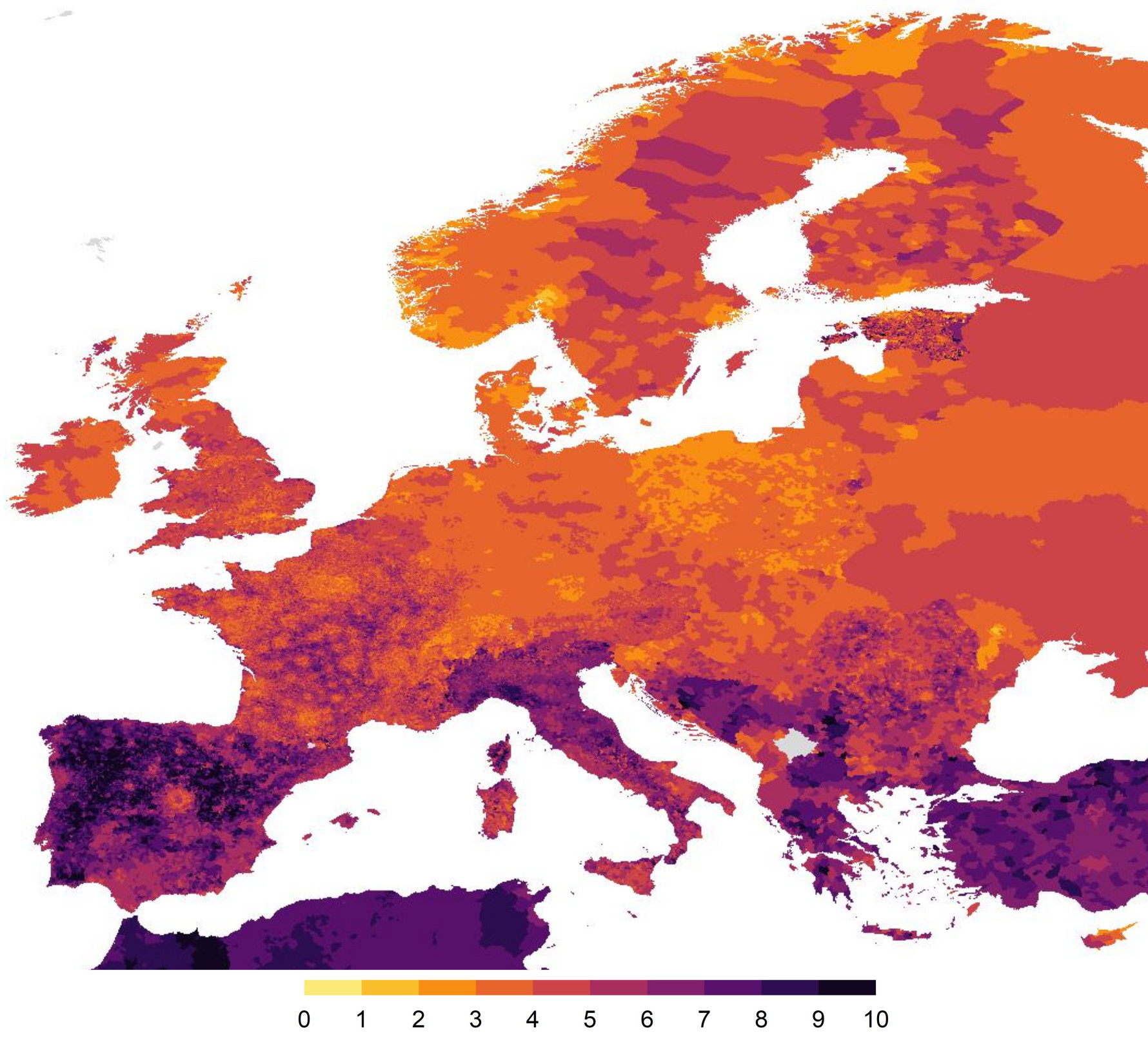
Fig. 12 The GlobE-SoVI for Europe (Reimann et al. 2024)

The assessment of physical vulnerability largely relies on damage curves, assuming that structures (e.g. buildings, infrastructure) will suffer a certain damage based on hazard intensity and structure materials. Damage curves can depend on the building physical characteristics, including construction material, size, height, and age as well as its use and contents (Davis, 1985; Marvi, 2020).

• Buildings: Building materials data can be used from the PAGER database (Jaiswal et al., 2010). A recent study assembled over 1,250 vulnerability curves for different types of critical infrastructure and hazards (i.e. flooding, earthquakes, windstorms and landslides) (Nirandjan et al., 2024).

• To assess agricultural crop vulnerability to drought, the GAEZ dataset (Fischer et al., 2021) representing the share of cropland equipped for full control irrigation (%) can be used as a proxy for physical vulnerability to the occurrence of droughts and, more in general, to precipitation scarcity for the agricultural sector. The dataset has global spatial coverage and is available for the reference year 2010 at 5 arc minutes resolution.

• Road networks from OSM data can be categorized into primary, secondary, and tertiary roads, representing varying levels of vulnerability to potential wildfires. This classification can be a proxy of the proximity of roads to wildland areas outside of urban centres, with higher vulnerability attributed to roads closer to such areas.

Additionally, a set of spatially explicit vulnerability maps are available from the JRC database, which encompasses population, ecological, and economic vulnerability (Figure 2). These maps, featuring percentile values, can be classified based on predefined thresholds to facilitate their utilisation in a risk contingency matrix (European Commission. Joint Research Centre., 2020). The index of population vulnerability is based on the population exposed in the vulnerable Wildland Urban Interface; the index of economic vulnerability is based on vegetation restoration cost, for forest and agriculture areas; the index of ecological vulnerability is based on the ecological “irreplaceability” score (IRR) of the local vegetation (weighted average IRR) and the protected area fraction (PAF) for each burnable grid cell. The three vulnerability rasters are available at 1 km spatial resolution in Lambert Azimuthal Equal Area projection (ETRS89-LAEA).

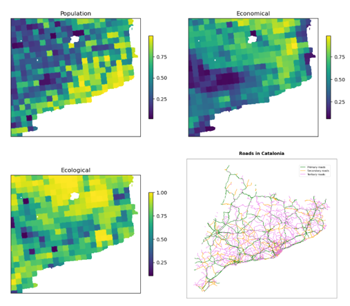
Fig. 13 Vulnerability data (population, economical, ecological) from JRC and roads colored by level of vulnerability from OSM, for the pilot area of Catalonia

Currently, hardly any future projections of social vulnerability characteristics are available at European scale. Several global studies produced projections of Gross Domestic Product (GDP) based on spatial population projections, e.g. at 0.5 degree, 0.25 degree, and 30 arc seconds spatial resolution. Future projections (2015-2050, 2050-2100) for GDP per capita and percentage of rural population are available as global grids at 30 arc-seconds resolution from Global CWatM. These data are aligned with the SSPs scenarios and are available upon request. Such projections can be used as a proxy for socioeconomic status.

Table 5 Pan-European future vulnerability projections datasets with technical specifications and advantages and disadvantages

Variable	Scenarios	Temporal resolution	Spatial resolution	References	Pros	Cons
Gross Domestic Product	SSPs 1-3	2010-2100	0.5 decimal degrees	(Murakami & Yamagata, 2019)	Proxy for future socioeconomic status	Low spatial resolution; three SSPs only
	SSPs 1-5	2005-2100	0.25 decimal degrees, 30 arcsec	(T. Wang & Sun, 2022)	Proxy for future socioeconomic status	Based on quite dated population projections
GDP/capita	SSPs 1, 3, 5	2015-2050, 2050-2100	30 arcsec	(Burek et al., 2020)	Global coverage	Dataset not public, but available upon request; three SSPs only
Rural population	SSPs 1, 3, 5	2015-2050, 2050-2100	30 arcsec	(Burek et al., 2020)	Global coverage	Dataset not public, but available upon request; three SSPs only

In addition to the spatial dataset described above, vulnerability is often assessed with the help of damage or mortality functions. For instance, damage curves assume that structures (e.g. buildings, infrastructure) will suffer a certain damage based on hazard intensity and structure materials. Therefore, building materials data can be used from the Pager database (Jaiswal et al., 2010). For flood vulnerability, damage curves are available for different buildings and land use types. The table below provides and overview of vulnerability functions for floods and heat stress, with more detail provided on the corresponding website.

Table 6 Damage or mortality functions

Name	Source	Hazard type	Exposure category	Model type	Scale
Global flood damage functions	(Huizinga et al., 2017)	Floods	Built-up	Damage funciton	Regional
Global flood mortality functions	(Jonkman & Vrijling, 2008)	Floods	Population	Mortality function	Global
Heat stress index classification	(Zare et al., 2019)	Heat stress	Population	Impact classification	Global