Risk assessment for heavy snowfall & blizzards#
A workflow from the CLIMAAX Handbook and SNOW GitHub repository.
See our how to use risk workflows page for information on how to run this notebook.
Risk assessment methodology#
The method involves visually representing the susceptible population exposed to intense snowfall and blizzards. This can be achieved by overlaying indicators for heavy snowfall and blizzards with population data. The objective is to understand the present probability of severe snowfall and blizzards, pinpointing the regions most impacted within Europe. Additionally, we seek to investigate how climate change may modify this exposure over time.
Blizzard#
A blizzard is a severe storm condition defined by low temperature, sustained wind or frequent wind gust and considerable precipitating or blowing snow. For blizzard conditions we propose the use of following impact indicator:
Blizzard days = Tmean ≤ 0 °C, Rs (snow amount) ≥ 10 cm and Wg (wind gust) ≥ 17 m/s (Vajda et al., 2014).
This impact indicator was defined taking into account the exposure of critical infrastructure, i.e., roads, rails, power lines, telecommunication to the hazard and is based on an extensive literature review, media reports, surveys conducted with European CI operators and case studies.
Heavy Snow#
Heavy snowfall may cause many disruptions and impacts in various sectors; however, the impacts and consequences of this hazard depend on the affected sector, infrastructure and also preparedness of society that varies over Europe. For example, already a few centimeters of snow can disrupt road traffic, but doesn’t normally cause any harm to energy infrastructure. Many weather services have three warning levels based on the severity of expected impacts, which are typically different for different sectors of infrastructure. There is a large variation in the national warning criteria or thresholds.
Similarly to blizzard, the impact indicators for heavy snowfall were defined taking into account the exposure of critical infrastructure, i.e., roads, rails, power lines, telecommunication to the hazard and is based on an extensive literature review, media reports, surveys conducted with European CI operators and case studies. The qualitative description of the two-level thresholds are:
1st threshold (> 6 cm): Some adverse impacts are expected, their severity depends on the resilience of the system, transportation is mainly affected.
2nd threshold (> 25 cm): The weather phenomena are so severe that is likely that adverse impact will occur, CI system is seriously impacted.
This code calculates the Annual probability (%) of a blizzard and heavy snowfall days during the specified period and a region of interest.
The annual probability
The annual probability is determined by dividing the count of events surpassing predefined thresholds within a year by the total number of days in that year. The result is then multiplied by 100 to express the probability as a percentage
P = ((variable > threshold) / days in year ) × 100
Preparation work#
Load libraries#
Find more info about the libraries used in this workflow here
warnings - To control the Python warning message
os - To create directories and work with files
pooch - To download and unzip the data
numpy - Numerical computing tools
xarray - To process the NetCDF data and prepare it for further calculation
rasterio - To access and explore geospatial raster data in GeoTIFF format
rioxarray - Rasterio xarray extension - to make it easier to use GeoTIFF data with xarray
matplotlib, cartopy - To plot the maps
localtileserver - To serve data to the interactive maps
import os
import warnings

import pooch
import numpy as np
import xarray as xr
import rioxarray as rxr
import rasterio

# Static map plotting
import matplotlib.pyplot as plt
import cartopy.crs as ccrs
import cartopy.feature as cfeature

# Interactive map plotting
import localtileserver
import folium
import branca
# Suppress some warnings that are repeatedly generated when browsing the interactive map
warnings.filterwarnings("ignore", message='invalid value encountered in cast')
warnings.filterwarnings('ignore', message='Adjusting dataset latitudes to avoid re-projection overflow')

# Set host forwarding for remote jupyterlab sessions
if 'JUPYTERHUB_SERVICE_PREFIX' in os.environ:
    os.environ['LOCALTILESERVER_CLIENT_PREFIX'] = os.path.join(os.environ['JUPYTERHUB_SERVICE_PREFIX'], 'proxy/{port}')
Select area of interest#
Before accessing the data, we will define the area of interest. Prior to commencing this workflow, you should have already prepared by downloading the heavy snowfall and blizzards hazard map to your local directory (using the SNOW hazard workflow for heavy snowfall and blizzards or by using your own data). Please specify the name of the area for the snow hazard maps below.
areaname = 'Europe'
Create the directory structure#
We need a directory structure for accessing and storing data.
If you have already executed the hazard assessment workflow, you have already created the workflow folder SNOW_hazard where the hazard data is stored.
We add additional data from this risk workflow notebook into the same folder.
workflow_folder = 'SNOW_hazard'
os.makedirs(workflow_folder, exist_ok=True)
data_dir = os.path.join(workflow_folder, f'data_{areaname}')
os.makedirs(data_dir, exist_ok=True)

plot_dir = os.path.join(workflow_folder, f'plots_{areaname}')
os.makedirs(plot_dir, exist_ok=True)

general_data_dir = os.path.join(workflow_folder, 'general_data')
os.makedirs(general_data_dir, exist_ok=True)
Step 1: Hazard data#
Intense snowfall and blizzards maps#
As default option, we use the intense snowfall and blizzards maps from the ERA5 single level dataset and CORDEX single level dataset, that were downloaded using the hazard assessment workflow for snow and blizzards. Below we load the maps and visualize them to check the contents.
Load EURO-CORDEX data#
Choose the parameters as in the Hazard workflow to pick up the data produced there.
Hist_start_year    = '1991'
Hist_end_year      = '1995'
Hist_experiment_in = 'historical'

RCP_start_year     = '2046'
RCP_end_year       = '2050'

experiment_names  = ['rcp_2_6', 'rcp_4_5', 'rcp_8_5']
experiment_names1 = ['rcp26', 'rcp45', 'rcp85']
# Select the RCP scenario you want to use
experiment_choice = 0

RCP_experiment_in  = experiment_names[experiment_choice]
RCP_experiment_in1 = experiment_names1[experiment_choice]

ensemble_member_in = 'r1i1p1'
# List of model names
gcm_extr_list = ['NCC-NorESM1-M', 'MPI-M-MPI-ESM-LR', 'CNRM-CERFACS-CNRM-CM5', 'NCC-NorESM1-M']
rcm_extr_list = ['GERICS-REMO2015', 'SMHI-RCA4', 'KNMI-RACMO22E', 'SMHI-RCA4']
# Select the global and regional climate model combination you want to use (count starts at 0)
model_choice = 1

gcm_model_Name = gcm_extr_list[model_choice]
rcm_model_Name = rcm_extr_list[model_choice]

# Filename suffixes
cordex_suffix_hist = f'{gcm_model_Name}_{rcm_model_Name}_{Hist_experiment_in}_{ensemble_member_in}_{Hist_start_year}_{Hist_end_year}'
cordex_suffix_fur = f'{gcm_model_Name}_{rcm_model_Name}_{RCP_experiment_in1}_{ensemble_member_in}_{RCP_start_year}_{RCP_end_year}'

print(RCP_experiment_in1)
print(gcm_model_Name)
print(rcm_model_Name)
rcp26
MPI-M-MPI-ESM-LR
SMHI-RCA4
Load CORDEX historical data
BdayCount_anaProb_mean_path = os.path.join(data_dir, f'BdayCount_AnaProb_mean_{cordex_suffix_hist}.nc')
BdayCount_anaProb_mean_hist = xr.open_dataarray(BdayCount_anaProb_mean_path, decode_coords='all')

snow6Prob_annual_mean_path = os.path.join(data_dir, f'Snow6Prob_annual_mean_{cordex_suffix_hist}.nc')
snow6Prob_annual_mean_hist = xr.open_dataarray(snow6Prob_annual_mean_path, decode_coords='all')

snow25Prob_annual_mean_path = os.path.join(data_dir, f'Snow25Prob_annual_mean_{cordex_suffix_hist}.nc')
snow25Prob_annual_mean_hist = xr.open_dataarray(snow25Prob_annual_mean_path, decode_coords='all')
Load CORDEX future data
BdayCount_anaProb_mean_path = os.path.join(data_dir, f'BdayCount_AnaProb_mean_{cordex_suffix_fur}.nc')
BdayCount_anaProb_mean_fur = xr.open_dataarray(BdayCount_anaProb_mean_path, decode_coords='all')

snow6Prob_annual_mean_path = os.path.join(data_dir, f'Snow6Prob_annual_mean_{cordex_suffix_fur}.nc')
snow6Prob_annual_mean_fur = xr.open_dataarray(snow6Prob_annual_mean_path, decode_coords='all')

snow25Prob_annual_mean_path = os.path.join(data_dir, f'Snow25Prob_annual_mean_{cordex_suffix_fur}.nc')
snow25Prob_annual_mean_fur = xr.open_dataarray(snow25Prob_annual_mean_path, decode_coords='all')
Load ERA5 data#
BdayCount_anaProb_mean_path = os.path.join(data_dir, f'BdayCount_AnaProb_mean_ERA5_{Hist_start_year}_{Hist_end_year}.nc')
BdayCount_anaProb_mean_ERA = xr.open_dataarray(BdayCount_anaProb_mean_path, decode_coords='all').rio.write_crs(4326)

snow6Prob_annual_mean_path = os.path.join(data_dir, f'Snow6Prob_annual_mean_ERA5_{Hist_start_year}_{Hist_end_year}.nc')
snow6Prob_annual_mean_ERA = xr.open_dataarray(snow6Prob_annual_mean_path, decode_coords='all').rio.write_crs(4326)

snow25Prob_annual_mean_path = os.path.join(data_dir, f'Snow25Prob_annual_mean_ERA5_{Hist_start_year}_{Hist_end_year}.nc')
snow25Prob_annual_mean_ERA = xr.open_dataarray(snow25Prob_annual_mean_path, decode_coords='all').rio.write_crs(4326)
Change in annual probability#
Compute change of hazard indicators
def change(hist, fur):
    return (fur - hist).where(hist > 1, other=0).drop_vars(['rotated_pole', 'height'])

BdayCount_anaProb_mean_change = change(BdayCount_anaProb_mean_hist, BdayCount_anaProb_mean_fur)
snow6Prob_annual_mean_change = change(snow6Prob_annual_mean_hist, snow6Prob_annual_mean_fur)
snow25Prob_annual_mean_change = change(snow25Prob_annual_mean_hist, snow25Prob_annual_mean_fur)
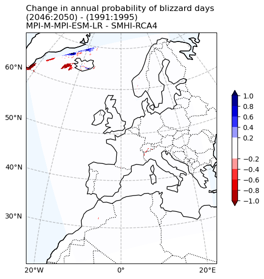
Change in Blizzard days probability#
fig, ax = make_map(
    'Change in annual probability of blizzard days\n'
    f'({RCP_start_year}:{RCP_end_year}) - ({Hist_start_year}:{Hist_end_year})\n'
    f'{gcm_model_Name} - {rcm_model_Name}'
)

plot_change(ax, BdayCount_anaProb_mean_change, max_level=1.)

fig.savefig(os.path.join(plot_dir, f'Chan_Ann_prob_blizzard_days_CORDEX_{cordex_suffix_fur}.png'))
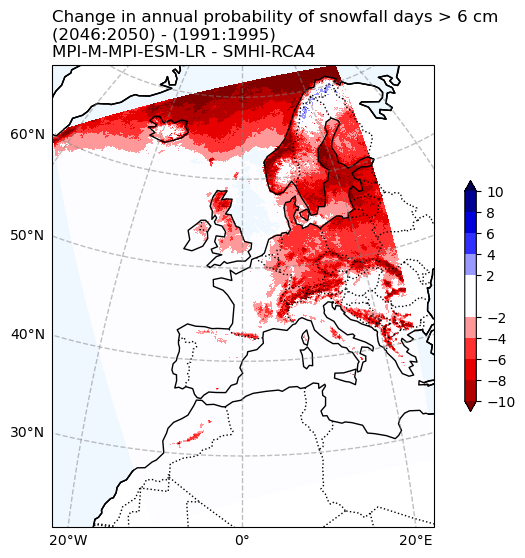
Change in snowfall days > 6 cm probability#
fig, ax = make_map(
    'Change in annual probability of snowfall days > 6 cm\n'
    f'({RCP_start_year}:{RCP_end_year}) - ({Hist_start_year}:{Hist_end_year})\n'
    f'{gcm_model_Name} - {rcm_model_Name}'
)

plot_change(ax, snow6Prob_annual_mean_change, max_level=10.)

fig.savefig(os.path.join(plot_dir, f'Chan_Ann_prob_snow_days_6_CORDEX_{cordex_suffix_fur}.png'))
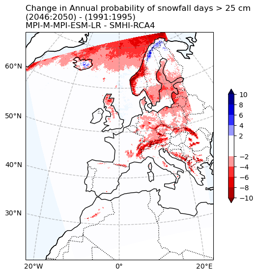
Change in snowfall days > 25 cm probability#
fig, ax = make_map(
    'Change in Annual probability of snowfall days > 25 cm\n'
    f'({RCP_start_year}:{RCP_end_year}) - ({Hist_start_year}:{Hist_end_year})\n'
    f'{gcm_model_Name} - {rcm_model_Name}'
)

plot_change(ax, snow25Prob_annual_mean_change, max_level=10.)

fig.savefig(os.path.join(plot_dir, f'Chan_Ann_prob_snow_days_25_CORDEX_{cordex_suffix_fur}.png'))
Step 2: Exposure data#
Download population data#
In this illustration, we are using population data sourced from the JRC data portal, specifically the Global Human Settlement Layer Global Human Settlement Layer GHSL, with 30 arcsec resolution global datasets. After downloading and extracting the data, Pooch will list the contents within the data directory.
pop_files = pooch.retrieve(
    url='https://jeodpp.jrc.ec.europa.eu/ftp/jrc-opendata/GHSL/GHS_POP_GLOBE_R2023A/GHS_POP_E2025_GLOBE_R2023A_4326_30ss/V1-0/GHS_POP_E2025_GLOBE_R2023A_4326_30ss_V1_0.zip',
    known_hash=None,
    path=general_data_dir,
    processor=pooch.Unzip(extract_dir=''),
    progressbar=True
)
The zip file contains data, as well as metadata and the documentation in the pdf file.
Load the data#
Population data is in file with filename: GHS_POP_E2025_GLOBE_R2023A_4326_30ss_V1_0.tif
We can use rioxarray to load this file and explore the projections of the dataset.
population_file = os.path.join(general_data_dir, 'GHS_POP_E2025_GLOBE_R2023A_4326_30ss_V1_0.tif')

population = xr.open_dataarray(population_file).squeeze()
population
<xarray.DataArray 'band_data' (y: 21384, x: 43202)> Size: 7GB
[923831568 values with dtype=float64]
Coordinates:
    band         int64 8B 1
  * x            (x) float64 346kB -180.0 -180.0 -180.0 ... 180.0 180.0 180.0
  * y            (y) float64 171kB 89.1 89.09 89.08 ... -89.08 -89.09 -89.1
    spatial_ref  int64 8B ...
Attributes:
    AREA_OR_POINT:             Area
    STATISTICS_MAXIMUM:        286330.44519772
    STATISTICS_MEAN:           8.8674048604304
    STATISTICS_MINIMUM:        0
    STATISTICS_STDDEV:         249.62729204313
STATISTICS_VALID_PERCENT: 100The population data has x and y as spatial dimensions, which are really longitude and latitude coordinates given in degrees.
population.rio.crs
CRS.from_epsg(4326)
The projection is WSG84/EPSG:4326.
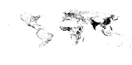
Quicklook#
The population dataset too big for us to reasonably visualise it in full at its original resolution. We will instead create a tile client for the dataset, which plots parts of the dataset on demand, so we can display it on an interactive map.
The tile client can create a quicklook for the dataset (this representation is coarsened):
pop_client = localtileserver.TileClient(population_file)
pop_client.thumbnail(vmin=0, vmax=100, colormap="binary")
Step 3: Visual overlay of hazard and exposure#
We want to overlay the population data on snowfall and blizzard indicators to better understand where these indicators affect densely populated areas.
# Map layers for orientation: light base and optional labels on top
layer_base = folium.TileLayer(
        "http://{s}.basemaps.cartocdn.com/light_nolabels/{z}/{x}/{y}.png",
        attr="CartoDB", control=False)
layer_labels = folium.TileLayer(
        "http://{s}.basemaps.cartocdn.com/light_only_labels/{z}/{x}/{y}.png",
        attr="Carto", overlay=True, control=True, name="Map labels", show=False)

# Population layer, clip at upper range (vmax), so smaller values remain visible
vmax_pop = 1000
layer_pop = localtileserver.get_folium_tile_layer(
        source=pop_client, colormap="binary", vmin=0, vmax=1000, nodata=0.0,
        name='Population', overlay=False, control=False)

colors_pop = plt.colormaps["binary"](np.linspace(0, 1.0, 51)).tolist()
colormap_pop = branca.colormap.LinearColormap(
        colors=colors_pop, vmin=0, vmax=vmax_pop, caption="Population [#/cell]")
def in_memory_tile_client(da):
    """Tile client from input data array"""
    mf = rasterio.MemoryFile()
    raster = mf.open(driver='GTiff', count=1, height=da.rio.height, width=da.rio.width,
            dtype=da.dtype, crs=da.rio.crs, transform=da.rio.transform(recalc=True),
            nodata=da.rio.nodata)
    raster.write(da.values, 1)
    raster.close()
    return localtileserver.TileClient(raster)
Population with historical snow indices (ERA5 reanalysis)#
def tile_client_for_era5(da):
    return in_memory_tile_client(
        da
    )

client_era_bday = tile_client_for_era5(BdayCount_anaProb_mean_ERA)
client_era_snow6 = tile_client_for_era5(snow6Prob_annual_mean_ERA)
client_era_snow25 = tile_client_for_era5(snow25Prob_annual_mean_ERA)

probability_style = {
    "vmin": 0,  # min value of colorbar
    "vmax": 50,  # max value of colorbar (adjust if necessary)
    "opacity": 0.5  # make layer semi-transparent so population data remains visible underneath
}

layer_era_bday = localtileserver.get_folium_tile_layer(
        source=client_era_bday, colormap="gnbu", **probability_style,
        name="Annual probability of blizzard days", overlay=False, show=False)
layer_era_snow6 = localtileserver.get_folium_tile_layer(
        source=client_era_snow6, colormap="gnbu", **probability_style,
        name="Annual probability of snowfall days > 6 cm", overlay=False, show=False)
layer_era_snow25 = localtileserver.get_folium_tile_layer(
        source=client_era_snow25, colormap="gnbu", **probability_style,
        name="Annual probability of snowfall days > 25 cm", overlay=False, show=True)

colors_prob = plt.colormaps["GnBu"](np.linspace(0, 1.0, 21)).tolist()
colormap_prob = branca.colormap.LinearColormap(
        colors=colors_prob, vmin=0, vmax=50, caption="Probability snowfall days [%]")
m = folium.Map(tiles=layer_base, location=[52, 10], zoom_start=4, control_scale=True)
m.add_child(layer_pop)
m.add_child(layer_era_bday)
m.add_child(layer_era_snow6)
m.add_child(layer_era_snow25)
m.add_child(layer_labels)
m.add_child(colormap_prob)
m.add_child(colormap_pop)
folium.LayerControl(collapsed=False).add_to(m)

print(f"ERA5 {Hist_start_year} to {Hist_end_year}")
print()
m
ERA5 1991 to 1995
Tip
Execute the notebook to see the data in the interactive map.
Population with change in snow indices (CORDEX projections)#
def tile_client_for_change(da, at_least=0.1):
    crs = ccrs.RotatedPole(pole_latitude=39.25, pole_longitude=-162)
    return in_memory_tile_client(
        da
        .where((da < -at_least) | (da > at_least))  # mask areas where change is small
        .drop_vars(["lat", "lon"])
        .rio.set_spatial_dims(x_dim="rlon", y_dim='rlat')
        .rio.write_crs(crs)
        .rio.write_nodata(np.nan)
        .rio.reproject("EPSG:4326")  # avoid issues with the rotated grid
    )

client_change_bday = tile_client_for_change(BdayCount_anaProb_mean_change)
client_change_snow6 = tile_client_for_change(snow6Prob_annual_mean_change)
client_change_snow25 = tile_client_for_change(snow25Prob_annual_mean_change)

change_style = {
    "vmin": -10,  # min value of colorbar
    "vmax": 10,  # max value of colorbar (adjust if necessary)
    "opacity": 0.5  # make layer semi-transparent so population data remains visible underneath
}

layer_change_bday = localtileserver.get_folium_tile_layer(
        source=client_change_bday, colormap="seismic_r", **change_style,
        name="Annual probability of blizzard days", overlay=False, show=False)
layer_change_snow6 = localtileserver.get_folium_tile_layer(
        source=client_change_snow6, colormap="seismic_r", **change_style,
        name="Annual probability of snowfall days > 6 cm", overlay=False, show=False)
layer_change_snow25 = localtileserver.get_folium_tile_layer(
        source=client_change_snow25, colormap="seismic_r", **change_style,
        name="Annual probability of snowfall days > 25 cm", overlay=False, show=True)

colors_prob = plt.colormaps["seismic_r"](np.linspace(0, 1.0, 21)).tolist()
colormap_prob = branca.colormap.LinearColormap(colors=colors_prob, vmin=-10, vmax=10,
        tick_labels=[-10, -5, 0, 5, 10], caption="Change in annual probability [%]")
m = folium.Map(tiles=layer_base, location=[52, 10], zoom_start=4, control_scale=True)
m.add_child(layer_pop)
m.add_child(layer_change_bday)
m.add_child(layer_change_snow6)
m.add_child(layer_change_snow25)
m.add_child(layer_labels)
m.add_child(colormap_prob)
m.add_child(colormap_pop)
m.add_child(folium.LayerControl(collapsed=False))

print(f"GCM: {gcm_model_Name}")
print(f"RCM: {rcm_model_Name}")
print(f"Change: ({RCP_start_year} to {RCP_end_year}) - ({Hist_start_year} to {Hist_end_year})")
print()
m
GCM: MPI-M-MPI-ESM-LR
RCM: SMHI-RCA4
Change: (2046 to 2050) - (1991 to 1995)
Tip
Execute the notebook to see the data in the interactive map.
Conclusions#
In this workflow, we’ve illustrated the process of exploring, processing, and visualizing data necessary for analyzing the influence of heavy snowfall and blizzard day indices on population density. These indices are presented as annual probabilities of occurrence, reflecting the likelihood of a particular event happening over several years. In the present climate, communities in the northern Alpine region face heightened vulnerability to heavy snowfall and blizzards. However, under the RCP2.5 scenario, we observe a significant reduction in the severity of these hazards across the region by mid-century compared to the current climate. Please note that this analysis is based on a single model and only 5 years of data. For greater accuracy, a 30-year period of data should be used, along with multi-model simulations to better account for model uncertainty.
Contributors#
Suraj Polade, Finnish Meteorological Institute
Andrea Vajda, Finnish Meteorological Institute