Hazard assessment for relative drought#
A workflow from the CLIMAAX Handbook and DROUGHTS GitHub repository.
See our how to use risk workflows page for information on how to run this notebook.
In this workflow, drought hazard (dH) for a given region is estimated as the probability of exceedance of the median of regional (e.g., EU level) severe precipitation deficits for a historical reference period (e.g. 1981-2015) or for a future projection period (e.g. 2031-2060; 2071-2100). The methodology used here was developed and applied globally by Carrão et al. (2016).
A workflow on how to quantify drought risk as the product of drought hazard, exposure and vulnerability can be found in the risk assessement notebook. Visualization tools based on preprocessed results for both drought hazard and drought risk can be found in the risk visualization notebook.
Below is a description of the data and tools used to calculate drought hazard, both for the historic period and for future scenarios, and the outputs of this workflow.
Input files#
This workflows requires monthly total precipitation for each NUTS3 region during the historical reference period or future projection period in a selected country.
Pre-processed data is available for the historic workflow as well as future projections. The ensamble average from ISIMIP 3b bias-adjusted atmospheric climate input data (https://doi.org/10.48364/ISIMIP.842396.1) is used for both historical period (1981 -2015) and future projections (near-future (2050) 2031 -2060 and far-future (2080) 2071 -2100). Precipitation data is the average of five CMIP6 global climate models (GCMs; GFDL-ESM4, IPSL-CM6A-LR, MPI-ESM1-2-HR, MRI-ESM2-0, UKESM1-0-LL), for three SSP-RCPs combinations (SSP126, SSP370, SSP585) provided at a spatial resolution of 0.5°x0.5°.
Note
The expected data format is a table where each row represents the total precipitation in mm for a month/year combination, and each column represents an area of interest (e.g. NUTS3 region). The first column contains the date in this format DD/MM/YYYY (Other formats shall be specified in the notebook by using the time_format = ‘%d/%m/%Y’ variable). The title of the first columns has to be ‘timing’ and the rest of the titles have to be the codes of the areas of interest (e.g. NUTS3), which have to be identical to the codes as they appear in the NUTS3 spatial data from the European Commission.
Tables with precipitation data were created for each dataset (historic and future projections) and saved as separate .csv files. Furthermore, for each of the selected SSP-RCPs combinations (SSP126, SSP370, SSP585) we created separate input files for the years 2031 -2060 (near-future) and 2071-2100 (far-future). Users are advised to use the provided data to preserve the consistency between the historical and projected data. Alternatively, users that prefer to use their precipitation data should make sure the historical and projected data are consistent (e.g., outputs of a single model).
Methodology#
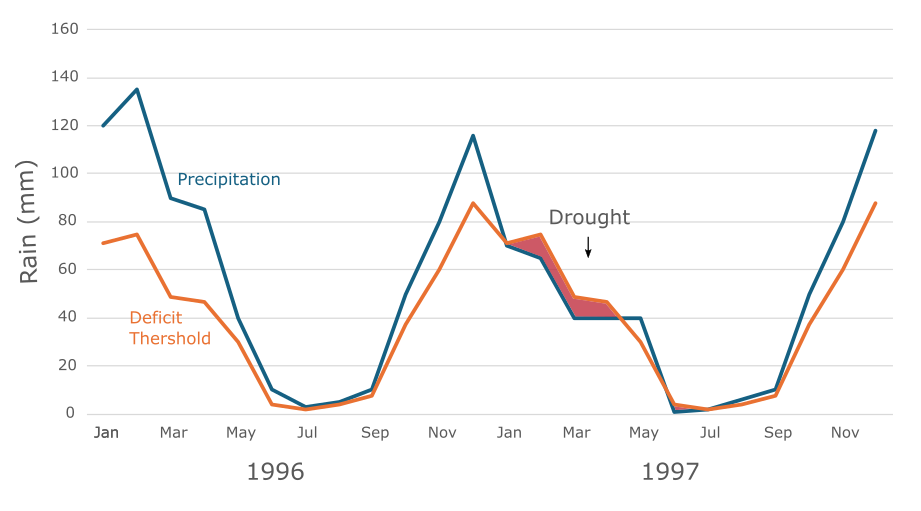
We use the weighted anomaly of standardized precipitation (WASP) index to define the severity of precipitation deficit. The WASP-index takes into account the annual seasonality of the precipitation cycle and is computed by summing weighted standardized monthly precipitation anomalies (see Eq. 1). Where \(P_{n,m}\) is each region’s monthly precipitation, \(T_m\) is a monthly threshold defining precipitation severity, and \(T_A\) is an annual threshold for precipitation severity. The thresholds are defined by dividing multi-annual monthly observed rain using the ‘Fisher-jenks’ classification algorithm.
Eq. 1:
Limitation#
For future scenarios, model uncertainity is not taken into account as we used an average of 5 different CMIP6 global climate models (GFDL-ESM4, IPSL-CM6A-LR, MPI-ESM1-2-HR, MRI-ESM2-0, UKESM1-0-LL) for each of the three SSP-RCPs combinations (SSP126, SSP370, SSP585). We recommended that users explore model uncertainty on our workflow on their own.
Workflow implementation#
Load libraries#
Find more info about the libraries used in this workflow here
import os
import pooch
os.environ['USE_PYGEOS'] = '0'
import pandas as pd
import numpy as np
import jenkspy
from datetime import date
Define working environment and global parameters#
This workflow relies on pre-processed data. The user will define the path to the data folder and the code below would create a folder for outputs.
# Set working environment
workflow_folder = './sample_data_nuts3/'

# Set time format of the 'timing' coloumn
time_format = '%d/%m/%Y'


# Define scenario 0: historic; 1: SSP1-2.6; 2: SSP3-7.0. 3: SSP5-8.5
scn = 0

# Define time (applicable only for the future): 0: near-future (2050); 1: far-future (2080)
time = 0

pattern = "historic"
pattern_h = "historic"
if scn != 0:
    pattern_h = ['ssp126', 'ssp370', 'ssp585'][scn - 1]
    pattern = ['ssp126', 'ssp370', 'ssp585'][scn - 1] + '_' + ['nf', 'ff'][time]

# debug if folder does not exist - issue an error to check path

# Create outputs folder
name_output_folder = 'outputs_hazards'
os.makedirs(os.path.join(workflow_folder, name_output_folder), exist_ok=True)
Access to sample dataset#
Load the file registry for the droughtrisk_sample_nuts3 dataset in the CLIMAAX cloud storage with pooch.
sample_data_pooch = pooch.create(
    path=workflow_folder,
    base_url="https://object-store.os-api.cci1.ecmwf.int/climaax/droughtrisk_sample_nuts3/"
)
sample_data_pooch.load_registry("files_registry.txt")
If any files requested below were downloaded before, pooch will inspect the local file contents and skip the download if the contents match expectations.
Choose country code#
Choose country code from:
‘HR’, ‘DE’, ‘BG’, ‘AT’, ‘AL’, ‘BE’, ‘ES’, ‘CH’, ‘CZ’, ‘EL’, ‘FR’, ‘FI’, ‘EE’, ‘DK’, ‘CY’, ‘HU’, ‘NL’, ‘NO’, ‘LV’, ‘LT’, ‘IS’, ‘MK’, ‘MT’, ‘IT’, ‘TR’, ‘PL’, ‘RO’, ‘SE’, ‘RS’, ‘PT’, ‘IE’, ‘UK’, ‘ME’, ‘LU’, ‘SK’, ‘SI’ ,‘LI’
ccode = "AL"
Load and visualize precipitation data#
# Download precipitation data for selected scenario
precip_file = sample_data_pooch.fetch(f"drought_hazard_{pattern_h}.csv")

print("Analyzing drought hazard. This process may take few minutes...")
print()

# Load precipitation data
precip = pd.read_csv(precip_file)
# Convert timing column to datetime
precip['timing'] = pd.to_datetime(precip['timing'], format= time_format)
#'%b-%Y'

# sort precip alphabetical order
precip = pd.concat([precip.iloc[:, 0], precip.iloc[:, 1:].reindex(sorted(precip.columns[1:]), axis=1)], axis=1)
# sort precip alphabetical order
# time  subset

if scn != 0:
    if time == 0:
        precip = precip.loc[(precip['timing'].dt.date >= date(2031,1,1)) & (precip['timing'].dt.date  < date(2060,1,1)), :]
    else:
        precip = precip.loc[(precip['timing'].dt.date >= date(2071,1,1)) & (precip['timing'].dt.date  < date(2100,1,1)), :]
else:
    precip = precip.loc[(precip['timing'].dt.date >= date(1981,1,1)) & (precip['timing'].dt.date  < date(2015,1,1)), :]

# col_subset aims to extract the relevant results
precip = precip.reset_index()

col_subset = list(precip.columns.str.contains(ccode))
col_subset[1] = True
precip = precip.loc[:, col_subset]

# clean NaN rows & missing columns
precip = precip.loc[~np.array(precip.isna().all(axis = 1)),:]

drop_regions = []

# missing data in columns
col_subset = np.array(precip.isna().all(axis = 0))
drop_regions += list(precip.columns[col_subset])
precip = precip.loc[:, ~col_subset]

regions = precip.columns[1:]
output = pd.DataFrame(regions, columns = ['NUTS_ID'])

print("The following regions are dropped due to missing data: "+ str(drop_regions))
print()
print('Input precipitation data (top 3 rows):')
print()
precip.head(3)
Analyzing drought hazard. This process may take few minutes...

The following regions are dropped due to missing data: []

Input precipitation data (top 3 rows):
| timing | AL011 | AL012 | AL013 | AL014 | AL015 | AL021 | AL022 | AL031 | AL032 | AL033 | AL034 | AL035 | |
|---|---|---|---|---|---|---|---|---|---|---|---|---|---|
| 0 | 1981-01-01 | 94.509786 | 103.177409 | 95.659491 | 118.158386 | 145.852112 | 95.855312 | 101.301849 | 109.709854 | 110.578285 | 113.682153 | 82.214381 | 120.947492 |
| 1 | 1981-02-01 | 99.241170 | 117.427653 | 94.274695 | 112.152197 | 124.374622 | 111.313041 | 114.888519 | 131.634750 | 135.891891 | 143.291309 | 87.761983 | 154.509487 |
| 2 | 1981-03-01 | 120.907837 | 131.979177 | 122.187512 | 142.389905 | 162.531689 | 126.032819 | 127.448021 | 147.864273 | 141.353043 | 168.668628 | 121.741007 | 172.366612 |
Calculate WASP Index (Weighted Anomaly Standardized Precipitation) monthly threshold#
# create empty arrays and tables for intermediate and final results
WASP = []
WASP_global = []
drought_class = precip.copy()


t_m = pd.DataFrame(np.zeros((12, len(precip.columns) - 1)))

for i in range(1, len(precip.columns)):

    # For every NUTS3 out of all regions - do the following:

    for mon_ in range(1, 13):
        # For every month out of all all months (January, ..., December) - do the following:

        # calculate monthly drought threshold -\
            # using a division of the data into to clusters with the Jenks' (Natural breaks) algorithm
        r_idx = precip.index[precip.timing.dt.month == mon_].tolist()

        t_m_last = jenkspy.jenks_breaks(precip.iloc[r_idx, i], n_classes = 2)[1]
        t_m.iloc[mon_ - 1, i - 1] = t_m_last


        # Define every month with water deficity (precipitation < threshold) as a drought month
        drought_class.iloc[r_idx, i] = (drought_class.iloc[r_idx, i] < t_m.iloc[mon_ - 1, i - 1]).astype(int)

    # calculate annual water deficit threshold

    t_a = list(t_m.sum(axis = 0))

    t_m0 = t_m.iloc[:, i - 1]
    t_a0 = t_a[i-1]
    # calculate droughts' magnitude and duration using the WASP indicator
    WASP_tmp = []
    first_true=0
    index = []
    for k in range(1, len(precip)):
        # for every row (ordered month-year combinations):
            # check if drought month -> calculate drought accumulated magnitude (over 1+ months)
        if drought_class.iloc[k, i]== 1:
            # In case of a drought month
            # calculate monthly WASP index
            index = int(drought_class.timing.dt.month[k] - 1)
            # WASP monthly index: [(precipitation - month_threshold)/month_threshold)]*[month_threshold/annual_treshold]
            WASP_last=((precip.iloc[k,i] - t_m0[index])/t_m0[index])* (t_m0[index]/t_a0)

            if first_true==0:
                # if this is the first month in a drought event:
                # append calculated monthly wasp to WASP array.
                WASP_tmp.append(WASP_last)
                first_true=1
            else:
                # if this is NOT the first month in a drought event:
                # add the calculated monthly wasp to last element in the WASP array (accumulative drought).
                WASP_tmp[-1]=WASP_tmp[-1] + WASP_last
            WASP_global.append(WASP_last)
        else:
            # check if not drought month - do not calculate WASP
            first_true=0
    WASP.append(np.array(WASP_tmp))
dH = []
WASP = np.array(WASP, dtype=object)
# calculate global median deficit severity -
    # set drought hazard (dH) as the probability of exceeding the global median water deficit.

median_global_wasp = np.nanmedian(WASP_global)

# calculate dH per region i
for i in range(WASP.shape[0]):
    # The more negative the WASP index, the more severe is the deficit event, so
    # probability of exceedence the severity is 1 - np.nansum(WASP[i] >= median_global_wasp) / len(WASP[i])
    if len(WASP[i]) > 0:
        # set minimum drought hazard as 0.05 to prevent the allocation of 0.0 to the regions with lowest hazard
        dH.append(np.maximum(round(1 - np.nansum(WASP[i] >= median_global_wasp) / len(WASP[i]), 3), 0.05))
    else:
        dH.append(0.05)


# https://agupubs.onlinelibrary.wiley.com/doi/pdf/10.1029/2004GL020901 - WASP Indicator description

output['wasp_raw_mean'] = [np.nan_to_num(np.nanmean(x), nan=0) for x in WASP]
output['wasp_raw_q25'] = [np.nan_to_num(np.nanquantile(x, q=0.25), nan=0) for x in WASP]
output['wasp_raw_median'] = [np.nan_to_num(np.nanmedian(x), nan=0) for x in WASP]
output['wasp_raw_q75'] = [np.nan_to_num(np.nanquantile(x, q=0.75), nan=0) for x in WASP]
output['wasp_raw_count'] = [x.shape[0] for x in WASP]

output['hazard_raw'] = dH
print('>>>>> Drought hazard is completed.')

output.to_csv(os.path.join(workflow_folder, name_output_folder, f'droughthazard_{ccode}_{pattern}.csv'),\
              index = False)
print('>>>>> Drought hazard indices were saved.')
>>>>> Drought hazard is completed.
>>>>> Drought hazard indices were saved.
Conclusions#
The above workflow calculates the drought hazard (dH) index that can be used as an input to calculate drought risk in the workflow described in the risk assessment notebook.
Users can use the WASP raw values as a measure of absolute drought hazard for the selected regions. Comparing WASP values of different NUTS3 regions of the selected country will help users understand how drought hazard might change in the future. Examples on how to do this can be found in the visualization workflow.
Contributors#
The workflow has beend developed by Silvia Artuso and Dor Fridman from IIASA’s Water Security Research Group, and supported by Michaela Bachmann from IIASA’s Systemic Risk and Reslience Research Group.
References#
[1] Carrão, H., Naumann, G., & Barbosa, P. (2016). Mapping global patterns of drought risk: An empirical framework based on sub-national estimates of hazard, exposure and vulnerability. Global Environmental Change, 39, 108-124.