Exercise#
How do we put our knowledge on climate scenarios and models into practice? In this exercise, we will explore the range of potential climate futures for your region and help you discover why these changes occur. These plausible changes are highlighted using individual climate model projections that can be reviewed for future weather patterns in one of the other CLIMAAX risk workflows.
We introduce each of the steps using a real-life example in Latvia. Be sure to expand the ‘Latvian example’ sections to see how we execute and interpret the steps for a real study:
Latvian example
For our example, we take the Lielupe basin, covering parts of Lithuania and Latvia. For Latvia, the basin has been characterised as a flood zone of national importance. See the figure below for an indication of the flood challenges in the region. Information on how these floods will develop in the future is of significant value as more and more adaptation plans and investments will need to be made as we head into the mid-century.
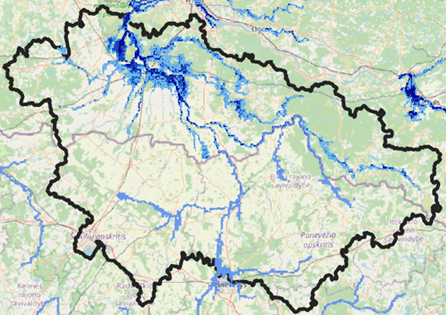
Fig. 22 Flood extent in the Lielupe Basin#
1. Define locally relevant climatic impact drivers#
Begin by identifying the specific climatic conditions that contribute to your climate-related challenge. The more specific you can be, the easier it will be to track changes and predict future hazards. Below is a set of key climate variables that can be explored on a yearly basis or for specific seasons.
Mean Temperature
Minimum Temperature
Minimum of Minimum Temperature
Frost Days
Heating Degree Days
Maximum Temperature
Maximum of Maximum Temperature
Days with Temperature > 35°C
Days with Temperature > 35°C (Bias Corrected)
Days with Temperature > 40°C
Days with Temperature > 40°C (Bias Corrected)
Cooling Degree Days
Total Precipitation
Maximum 1-Day Precipitation
Maximum 5-Day Precipitation
Consecutive Dry Days
Standardized Precipitation Index (6 months)
Total Snowfall
Surface Wind Speed
Note
Some of the variables above are accumulated (e.g., total precipitation, frost days), some are averaged (e.g., mean temperature, minimum temperature) and some characterize short-term extremes (e.g., minimum of minimum temperature, maximum 1-day precipitation). The choice of indicator should align with the desired application.
Latvian example
In Latvia, flooding is primarily driven by two factors. One is the snowpack accumulated in winter that rapidly melts and the melt water flows into rivers during spring. Another driver is spring precipitation, which saturates the soil and when this soil is confronted with extra rainfall, the region starts to flood.
To analyse developments for the two flood mechanisms we select the following climate impact drivers: Average precipitation March till May and Snowfall in December till February.
2. Collect observation trends from the interactive climate atlas#
To get a better understanding of what climate trend we can expect we will explore what climate trend is already observed. But before we begin we need to define our region using the IPCC climate zones. The IPCC divides Europe into four climatic zones. These zones are based on areas with similar climate typologies. For each of these zones, climate projection statistics are available.
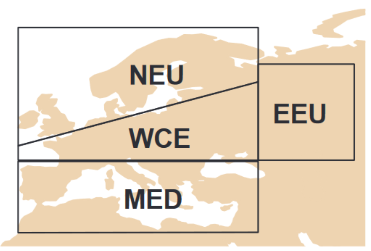
Fig. 23 IPCC climate zones in Europe. IPCC Atlas#
NEU - Northern Europe
WCE - West and Central Europe
MED - Mediterranean
EEU - Eastern Europe
We analyse past climate behaviour by following the next steps:
Select your region
Select the historical observation data set “era5-land”
Select climate impact drivers and season of interest
Click on “Regional Information” for more information
Spot potential trends
Latvian example
As Latvia is situated on the border between NEU and WCE we need to choose which region. Since the European risk assessment considers the Baltic states to be part of NEU we also choose this region. Overall, there has been an upward trend in ERA5 data for precipitation as can be seen from the graph.
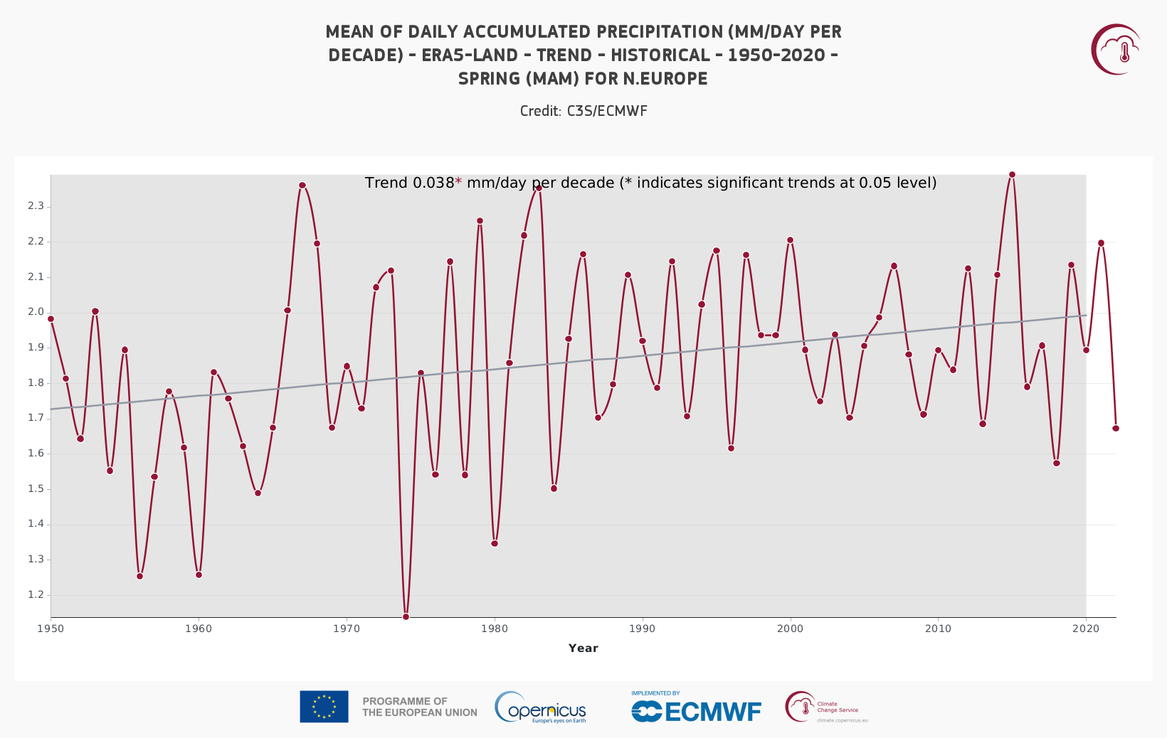
Fig. 24 Precipitation trend in spring for NEU (https://atlas.climate.copernicus.eu/atlas)#
In the whole of NEU we find that snow has a slightly increasing trend. The increasing rainfall trend might have contributed to more snow accumulation than temperature increases have reduced snow accumulation.
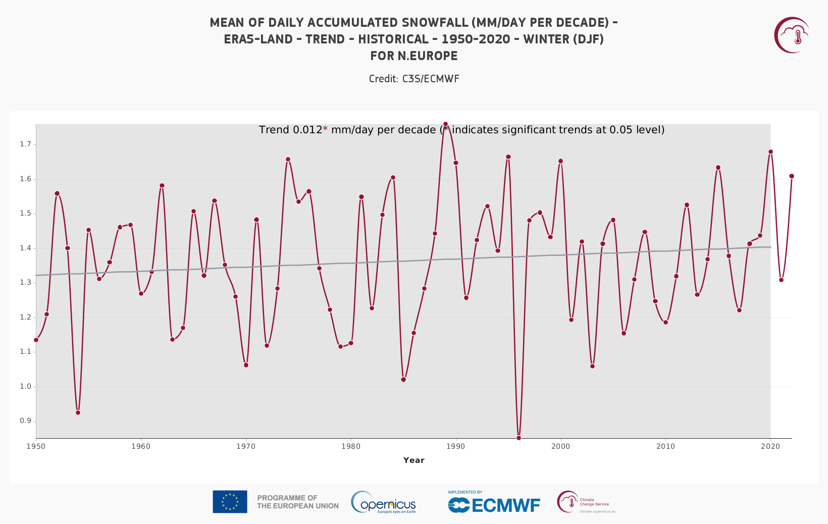
Fig. 25 Snow trend in winter in NEU (https://atlas.climate.copernicus.eu/atlas)#
Based on the above graphs, we would expect an increase in flood hazard associated with both the snowmelt and spring rainfall resulting in saturated soil.
3. Climate scenarios dashboard#
Use our climate scenarios dashboard to collect information on simulation trends.
Latvian example
Fig. 26 is obtained by selecting the change in Total Precipitation for the season Mar-May for the year 2041 for the NEU region. We notice that that the individual model projections span a much larger range of change than the SSP averaged scenarios. Here we see that individual models behave differently towards the same emission scenarios. This can be either due to differences in the way they represent physical processes or because they are subject to randomness of the weather and might have hit a cold snap or dry spell in their simulations.
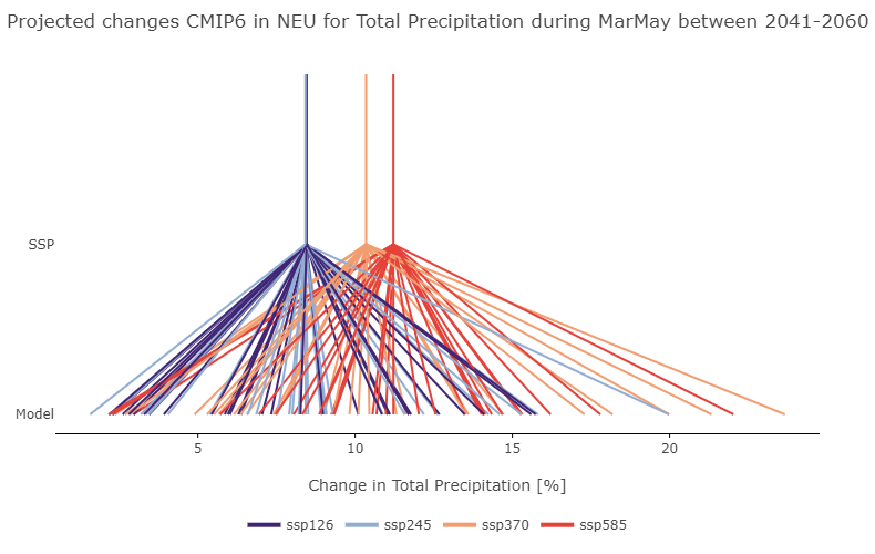
Fig. 26 Plot of uncertainties for climate variable in NEU#
Looking at changes in accumulated total precipitation over the spring season, we see that high-emission scenarios result in larger mean increases in precipitation (mean change across climate models). Projections based on individual climate models are ranging widely – some models show minor increase (<5%), while other models show much larger change (>15% in high-emission scenarios). When using this information with known flood mechanisms where soils are saturated and extra rain leads to high discharges, we can expect more of these events to occur. An increase of 10% extra precipitation in the spring season is not unlikely across models and can lead to severe changes in discharges.
Snowfall (Fig. 27) is expected to decrease when emissions, and thus also temperatures, increase. Given that Northern Europe historically received roughly 1.3 mm/day of snow in winter the range given is between a 24% reduction to a 7% increase in snowfall. Few models project an increase and this might only be due to randomness of weather. However, 7% extra snowfall in winter snowpack can result in large changes in melt discharges and might be worth investigating as a potential ‘what if’ scenario. A reduction of 24% is also interesting as it greatly limits snow accumulation and therefore the snow melt flood mechanism.
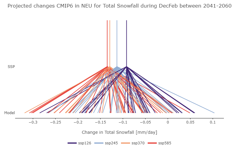
Fig. 27 Plot of uncertainties for climate variable in NEU#
4. Look into IPCC reports why this occurs#
To get a better sense of why there is such a large range of what could happen in the future we can dive into the IPCC reports to give some clarity. In the reports a scientific background is given to many of the projected changes. Here are some useful links: